Chapter 16 Variance Homogeneity - Many groups
Generally we are interested in testing whether or not there is a difference in the group means. When testing for differences in group means the specific test statistic formula to use depends on whether or not the group variances are equal. There is one formula for the case when the groups have equal variance, and a second formula to use when the group variances are not equal. When we are comparing two groups we use a variance ratio test. When there are multiple groups a possible test of whether the group variances are all equal is the Bartlett test.
16.1 The Bartlett Test
For the Bartlett test, the null hypothesis is that all the group variances are the same. The alternate hypothesis is that at least one of the group variances is different. The formula to calculate the test statistic is complicated, but it is still possible to obtain an intuitive understanding of the way the test works. The test works by comparing the variance calculated when the data are pooled together to form a single group to the variance calculated separately for each group. If the differences between the variance for each group and the pooled variance are large the conclusion drawn is that the group variances are not the same. The test statistic follows the chi-square distribution, but to determine what constitutes a `large’ value for the differences we use the the p-value decision rule. The null hypothesis that all the group variances are equal is rejected when the p-value is small.
16.2 Equal Variance Testing - Multiple Groups
To illustrate the test We will use the base R data set chickwts. This data set comes installed with R, which means we do not have to read in the data first. The data set has the weights of chickens that are on six different diets (feed regimes). Here we will be testing whether or not is appropriate to assume the variance for all six groups is the same using the Bartlett test function bartlett.test().
# Normally we would need to read the data in first but in this instance it is
# loaded already
str(chickwts)  # the data are in long format
#> 'data.frame':    71 obs. of  2 variables:
#>  $ weight: num  179 160 136 227 217 168 108 124 143 140 ...
#>  $ feed  : Factor w/ 6 levels "casein","horsebean",..: 2 2 2 2 2 2 2 2 2 2 ...
summary(chickwts)
#>      weight           feed
#>  Min.   :108   casein   :12
#>  1st Qu.:204   horsebean:10
#>  Median :258   linseed  :12
#>  Mean   :261   meatmeal :11
#>  3rd Qu.:324   soybean  :14
#>  Max.   :423   sunflower:12
Note the data structure. Can you see that there are six different feed types? Can you see how many observations there are per group? When the data are in long format the 5-number summary information ignores the grouping structure, so until we create a boxplot it is difficult to understand the nature of the data from just the summary information. One of the advantages of using the long format for data management with many groups is that it makes it easier to create a boxplot.
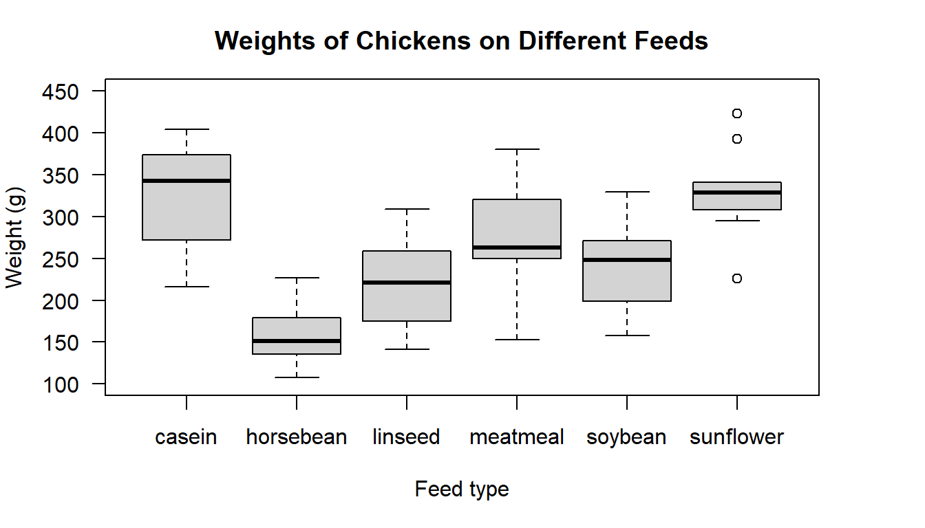
Figure 16.1: Boxplot of chicken weight distributions from six different feed types
Based on the boxplot, do the variances look equal? There definitely looks to be some difference in the means, but we cannot appropriately test the means before knowing if all the group variances are equal.
There appears to be some difference between the group variances, particularly with the sunflower feed, but remember we also have a fairly small number of observations in each group. Also note that for the sunflower group several `outliers’ have been identified. These values will work to increase the variance estimate. Overall, the difference in the spread of observations between groups does not look extreme. Based on this plot I would not be surprised if the formal test said it was safe to assume the group variances are equal.
Let’s run our test.
Step 1: Set the Null and Alternate Hypotheses
- Null hypothesis: The variance is the same for all groups
- Alternate hypothesis: The variance is not the same for all groups
- Null hypothesis: The variance is the same for all groups
Step 2: Implement Bartlett Test
For the test we specify the continuous and factor variable separated by a “\(\sim\),” in this order, because the data are in long format. Our alpha will be set as the default: 0.05.
with(chickwts, bartlett.test(weight ~ feed))  # long data format, use ~ not ,
#>
#>    Bartlett test of homogeneity of variances
#>
#> data:  weight by feed
#> Bartlett's K-squared = 3, df = 5, p-value = 0.7
Step 3: Interpret the Results
From the output we see the p-value = 0.66. Since 0.66 is greater than 0.05 (alpha), we:
Fail to reject the null hypothesis that the group variances are the same.What does this mean? It means, we have do not have sufficient evidence to say the variance is different across the groups. The test output also reports a K-squared value (3.26). Technically this is the test statistic - and it is this value we have used the p-value decision rule to conclude is not large. The df (5) represents our degrees of freedom, or the number of levels we have minus 1 (6 feeds - 1 = 5). As large values for the test statistic lead to a rejection of the null, we know that in this instance (3.26) is not large.
If we were to move on to conduct an ANOVA test to look for differences in the group means, we would conduct the test using the assumption that the group variances are equal. Using the function oneway.test(), this means we set the parameter var.equal to TRUE. If we reject the ANOVA test null hypothesis and move on to pair-wise t-tests then we would set the parameter pool.sd to TRUE when using the pairwise.t.test() function.
16.3 Advanced: Technical Note
As with the variance ratio test there are some known issues with the Bartlett test. For example, when the distributions are more peaked than a normal distribution (leptokurtic) the true alpha level is greater than the stated alpha level of the test. The chance of making a type I error is therefore higher than we think. Conversely, with distributions that are less peaked than a normal distribution (platykurtic) the true alpha level is less than the stated alpha level of the test, so the chance of making a type II error is increased. No relatively accessible reference for this issue has been identified, but a classic (relatively technical) reference that covers the issues is provided below.
For those interested in robust tests there are alternative tests that can be used. For example, there is Levene’s test, which is available in the car package; and also the non-parametric Fligner-Killeen test. Details on these tests can be obtained from the R help pages.
Reference
Box, G. E. (1953). Non-normality and tests on variances. Biometrika, 40(3/4), 318-335. https://www.jstor.org/stable/2333350