Chapter 12 Two Sample t-Test
Comparing two groups and testing whether the means of the two groups are different is a common process in science. However, rather than jump straight into the t-test it is necessary to follow a structured process of investigation. The structured process involves:
- A visual inspection of the data;
- A variance ratio pre-test, and
- The actual two sample t-test.
12.1 Example with Wide Format Data
For this example we have some phytoremediation data. Phytoremediation is the use of plants for remediating contaminated soil and water. Plant species are selected based on their ability to uptake or stabilize specific contaminants at a site, and this method of remediation is often preferred because it is low cost and relatively non-invasive.
Here we will look at the efficiency of two crop plants (redbeet and barley) at removing cadmium from the top 20 cm of soil at a contaminated site. The data we have is the percent reduction of cadmium after one harvest. Let’s read in our data and have a look at it before we conduct our test. Generally you will start by reading in the data from a .csv file or a .txt file. So that the work is reproducible, here we enter the data directly.
str() and summary() commands, here we also use the head() command to look at the data we have. The head() command shows the first six rows of the data, and is an easy way to see the data structure.
# read in our data (wide format)
Cd.BeetBarley<- data.frame(
  redbeet= c(18, 5, 10, 8, 16, 12, 8, 8, 11, 5, 6, 8, 9, 21, 9),
  barley= c(8, 5, 10, 19, 15, 18, 11, 8, 9, 4, 5, 13, 7, 5, 7))
# three ways to look at the data structure
str(Cd.BeetBarley)
#> 'data.frame':    15 obs. of  2 variables:
#>  $ redbeet: num  18 5 10 8 16 12 8 8 11 5 ...
#>  $ barley : num  8 5 10 19 15 18 11 8 9 4 ...
summary(Cd.BeetBarley)
#>     redbeet         barley
#>  Min.   : 5.0   Min.   : 4.0
#>  1st Qu.: 8.0   1st Qu.: 6.0
#>  Median : 9.0   Median : 8.0
#>  Mean   :10.3   Mean   : 9.6
#>  3rd Qu.:11.5   3rd Qu.:12.0
#>  Max.   :21.0   Max.   :19.0
head(Cd.BeetBarley)
#>   redbeet barley
#> 1      18      8
#> 2       5      5
#> 3      10     10
#> 4       8     19
#> 5      16     15
#> 6      12     18
Once we understand the data structure, and are confident the data has been read into R correctly, we then create a boxplot to look at the data. Remember, the boxplot is essentially a visual representation of the information we get with the summary() command.
with(Cd.BeetBarley,boxplot(redbeet,barley,
     col= "lightgrey",
     main= "Phytoremediation Efficiency of Crop Plants",
     xlab= "Crop type", ylab= "Cadmium reduction (%)",
     names= c("Redbeet","Barley"),
     ylim=  c(0,25), las= 1,
boxwex=0.6)) 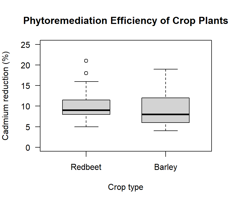
Figure 12.1: Box plot comparing the phytoremediation efficiency of redbeet and barley crop plants for removing cadmium from contaminated soil at depths of 0 to 20 cm
What do you see? Do the means looks different; does it look like we have equal variances? Looking at the data is a very important step in the process.
To determine which Two Sample t-test formula to use – equal variance formula or unequal variance formula – we need to compare the group variances. The Null hypothesis for the test is that the ratio of the two group variances is equal to one (they are equal); the Alternate hypothesis is that the ratio of the two group variances is not equal to one (they are not equal). For a more in-depth explanation of the variance ratio test see the reference guide for Variance Ratio Testing in R.
Before we conduct the actual variance ratio test, it is worth thinking through what we know about the data samples based on the data summary and the visual plot. From the data summary we know that we only have 15 observations in each group. On average, the more observations we have the more likely we are to reject the null. So, with few observations, if we are to reject the null the difference between the variance of each group will need to be substantial. From the boxplot we see that the “box” for redbeet looks a bit smaller than for barley. That suggests the variance for the redbeet sample might be smaller than for barley. On the other hand, we can also see that there are two “outliers” for the redbeet sample. These outliers’ values work to increase the variance, and so work to increase the variance estimate for redbeet. So based on a general understanding of the data samples we would not be surprised if, at the end of the formal test we conclude: do not reject the null.
with(Cd.BeetBarley, var.test(redbeet, barley))
#>
#>  F test to compare two variances
#>
#> data:  redbeet and barley
#> F = 1, num df = 14, denom df = 14, p-value = 1
#> alternative hypothesis: true ratio of variances is not equal to 1
#> 95 percent confidence interval:
#>  0.329 2.916
#> sample estimates:
#> ratio of variances
#>              0.979
From the output we see the p-value = 0.969 is greater than 0.05, so we:
Fail to reject the null hypothesis that the variance ratio is equal to one.
If we look at the actual ratio of the variances we see that it is 0.98. As such, are you surprised that we do not reject the null that the ratio is one? The practical implication of this for us is that we need to set our t-test parameter var.equal to TRUE.
Now let’s run our formal Two Sample t-test:
Step 1: Set the Null and Alternate Hypotheses
- Null hypothesis: The means of both groups are equal
- Alternate hypothesis: The means of both groups are not equal
Step 2: Implement the Two Sample t-test
Here we set
var.equalto TRUE, and leave alpha as the default, 0.05.Note: it is worth paying attention to the structure of the t-test when you have data in wide format.
with(Cd.BeetBarley, t.test(redbeet, barley, var.equal = TRUE))
#>
#>    Two Sample t-test
#>
#> data:  redbeet and barley
#> t = 0.4, df = 28, p-value = 0.7
#> alternative hypothesis: true difference in means is not equal to 0
#> 95 percent confidence interval:
#>  -2.87  4.20
#> sample estimates:
#> mean of x mean of y
#>      10.3       9.6
Step 3: Interpret the Results
From the output we see the p-value = 0.702. Since 0.702 is greater than 0.05 (alpha), we: Fail to reject the null hypothesis that the means are equal.
In other words: We do not have sufficient evidence to say the mean percent reduction of cadmium in soil at our site is different for our two crops (redbeet and barley). If you were trying to determine which plant to use to remediate a particular site, you would likely look to other factors, such as cost, environmental conditions or additional contaminants to be removed, to assist you in making your decision. Our output also provides the 95% confidence interval (-2.9, 4.2) for the actual difference between the means. Because the interval includes zero we get a non-significant p-value. Also note that the test output reports our group means (10.3, 9.6), which are the same as were given when we used the
str()command.
12.2 Example with Long Format Data
In this example, we will use a similar data set, but compare two different crops (maize and cabbage) which are known for their ability to remove cadmium from greater soil depths (20 to 40 cm). We will follow the same process as before, but this time our data will be in long format. This means when specifying our data we list our continuous variable (% Cd reduction) and factor variable (crop type) separated by a tilde, \(\sim\), rather than a comma.
# read in our data (long format)
Cd.CabbageMaize <- data.frame(remed.pcnt = c(46, 50, 44, 44, 43, 52, 48, 24, 51,
    29, 53, 32, 61, 59, 35, 34, 26, 44, 17, 34, 19, 34, 34, 43, 18, 34, 27, 27, 53,
    30), plt.typ = c(rep("cabbage", times = 15), rep("maize", times = 15)))
# get summary & check data structure
str(Cd.CabbageMaize)
#> 'data.frame': 30 obs. of 2 variables:
#> $ remed.pcnt: num 46 50 44 44 43 52 48 24 51 29 ...
#> $ plt.typ : chr "cabbage" "cabbage" "cabbage" "cabbage" ...
summary(Cd.CabbageMaize)
#> remed.pcnt plt.typ
#> Min. :17.0 Length:30
#> 1st Qu.:29.2 Class :character
#> Median :34.5 Mode :character
#> Mean :38.2
#> 3rd Qu.:47.5
#> Max. :61.0
head(Cd.CabbageMaize)
#> remed.pcnt plt.typ
#> 1 46 cabbage
#> 2 50 cabbage
#> 3 44 cabbage
#> 4 44 cabbage
#> 5 43 cabbage
#> 6 52 cabbageSo we will be working with data that is in two columns. But unlike the wide data format, the first column holds the numerical values for each group, and the second column holds the grouping information (what type of plant). The way the data is structured has implications for the commands we use to create plots and conduct tests.
# Note we don't NEED to give names for boxes if the data is in long format
# This is an advantage of the long format approach
with(Cd.CabbageMaize,boxplot(remed.pcnt~plt.typ,
     col= "lightgrey",
     main= "Phytoremediation Efficiency of Crop Plants",
     xlab= "Crop type", ylab= "Cadmium reduction (%)",
ylim= c(10,70), las= 1, boxwex=.6)) 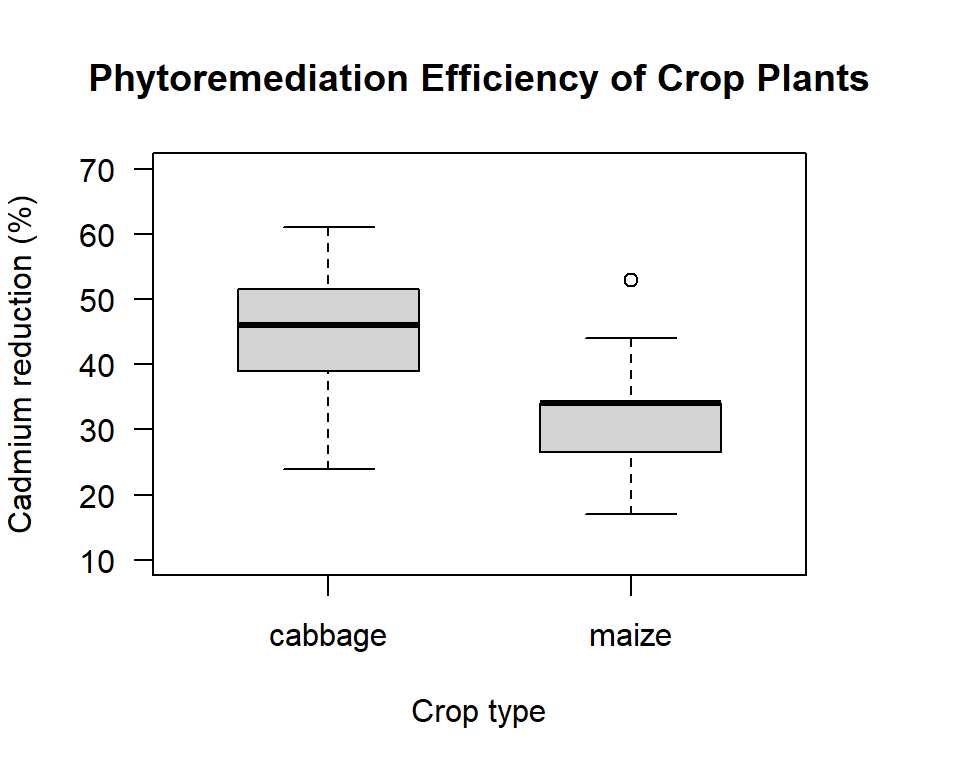
Figure 12.2: Box plot comparing the phytoremediation efficiency of cabbage and maize crop plants for removing cadmium from contaminated soil at depths of 20 to 40 cm.
Here the variances do not look that different. The box part of the plot for maize is smaller than for cabbage, but with the outlier for the maize crop working to increase the variance estimate for this group, I would not be surprised if the formal test says it is safe to assume the group variances are the same. As before, our Null hypothesis is that the variance ratio is equal to one (they are equal), and our Alternate hypothesis is that the variance ratio is not equal to one (they are not equal).
with(Cd.CabbageMaize, var.test(remed.pcnt ~ plt.typ))  # long format, use ~ not ,
#>
#>  F test to compare two variances
#>
#> data:  remed.pcnt by plt.typ
#> F = 1, num df = 14, denom df = 14, p-value = 0.8
#> alternative hypothesis: true ratio of variances is not equal to 1
#> 95 percent confidence interval:
#>  0.384 3.410
#> sample estimates:
#> ratio of variances
#>               1.14
From the output we see the p-value = 0.804, is greater than 0.05, so again we:
Fail to reject the null hypothesis that the variance ratio is equal to one and set our t-test parameter var.equal to TRUE. Again, if we look at the actual variance ratio number (1.14) we should not be surprised that we fail to reject the null: the value is quite close to one.
Now let’s run our formal Two Sample t-test:
Step 1: Set the Null and Alternate Hypotheses
- Null hypothesis: The group means are equal
- Alternate hypothesis: The group means are not equal
- Null hypothesis: The group means are equal
Step 2: Implement the Two Sample t-test
Here we set
var.equalto TRUE, and leave alpha as the default, 0.05.
with(Cd.CabbageMaize, t.test(remed.pcnt ~ plt.typ, var.equal = TRUE))
#>
#>  Two Sample t-test
#>
#> data:  remed.pcnt by plt.typ
#> t = 3, df = 28, p-value = 0.002
#> alternative hypothesis: true difference in means is not equal to 0
#> 95 percent confidence interval:
#>   5.38 20.89
#> sample estimates:
#> mean in group cabbage   mean in group maize
#>                  44.7                  31.6
Step 3: Interpret the Results
From the output we see the p-value = 0.002. Since 0.002 is less than 0.05 (alpha), we:
Reject the null hypothesis that the means are equal.
In other words: We have sufficient evidence to say the mean percent reduction of cadmium in soil at our site is higher for cabbage than for maize. This is an important piece of information, but it is not the only piece of relevant information. You will also need other information, such as whether or not there are any differences in establishment costs for each plant. You would also always refer back to the group means (44.7, 31.6%) and your confidence interval (5.4, 20.9%). Does a difference of about 13 percentage points matter in your situation? What about if the difference is only 5 percentage points (lower end of your 95% C.I.)? Your statistical test results are just numbers until you logically apply them to your research question, and the accepted methods of your research discipline.
# Two sample t-test: Extension Material