Chapter 11 Variance Ratio Test
Generally we are interested in testing whether or not there is a difference in the group means. When testing for differences in group means the specific test statistic formula to use depends on whether or not the group variances are equal. There is one formula for the case when the groups have equal variance, and a second formula to use when the group variances are not equal. Sometimes we are just interested in knowing whether or not the variance of two groups is different. For example, if we invest in a glasshouse to grow plants we would expect the variation in plant development to be less than for plants grown in the field.
When there are only two groups the test we use to determine if the variance is the same is called a variance ratio test. The test involves dividing the variance of group one by the variance of group two. If this ratio is close to one the conclusion drawn is that the variance of each group is the same. If the ratio is far from one the conclusion drawn is that the variances are not the same.
How far from one would this ratio need to be before we are convinced that the two population variances are not equal? In the case where the variable that we are interested in follows a normal distribution in the two populations, and these normal distributions have the same variance, then the ratio of sample variances follows another known distribution, known as the \(F\)-distribution. In the standard notation \(S^2_1\) and \(S^2_2\) are the sample variances from population \(1\) and population \(2\) respectively, then the ratio \[F=S^2_1/S^2_2\] follows an \(F\)-distribution when then population variances are equal. The only two parameters of the \(F\)-distribution are the degrees of freedom. These are related to the sizes of the samples taken from the two populations, \(m\) and \(n\). The way that the shape of the \(F\)-distribution changes with different degrees of freedom is shown in Figure .
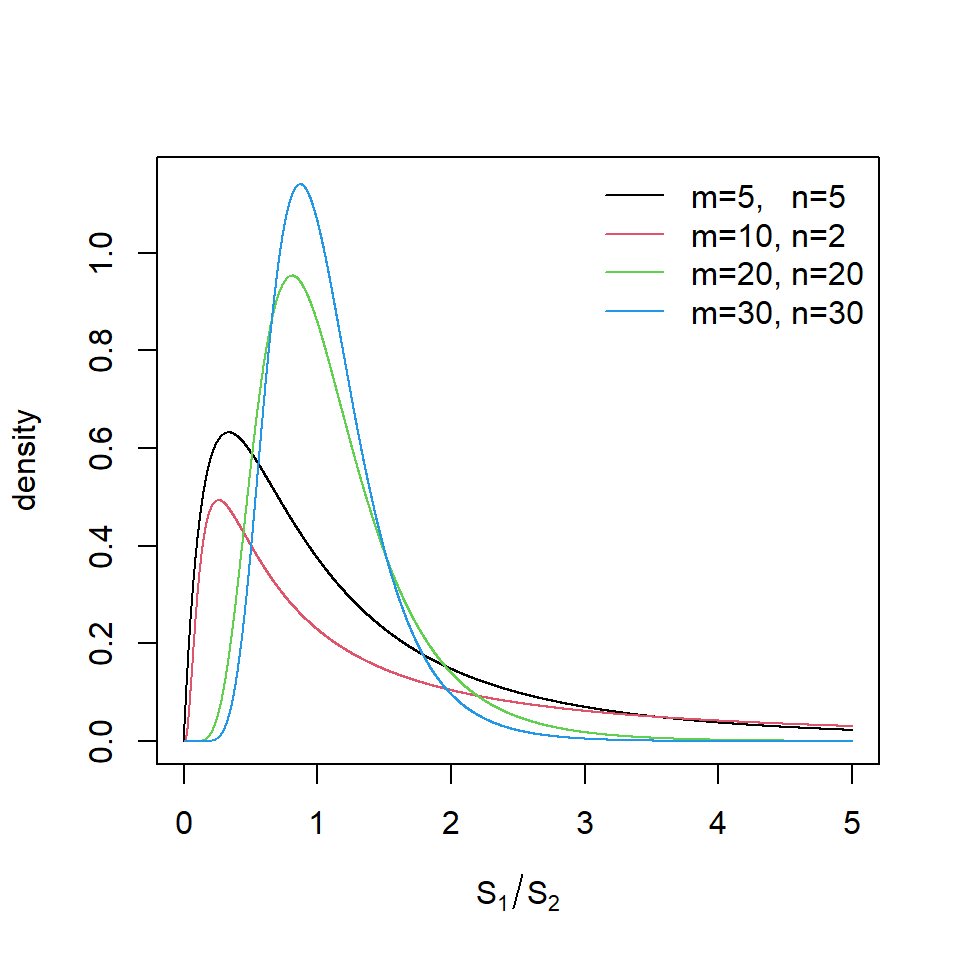
Figure 11.1: F-distribution for varying degrees of freedom
You’ll notice that as the sample sizes increase, the shape of the distribution gets more closely centred around one. This means that as our sample variances are based on more observations, the ratio of sample variances doesn’t need to stray as far from one in order for us to declare that the population variance are not equal. To put this another way, if we only take small samples from each population, our sample variance estimates won’t be very good and so we could belive that the ratio of the two sample variances might be quite different to one, just by chance. As we increase the sample taken from each population we are more certain that the sample variances are close to the population variances and so if the ratio was only a small distance from one, we would no longer believe that the population variances were equal.
To determine what values are close to one and what values are far from one we use the p-value decision rule. For the variance ratio test the null hypothesis that the group variances are equal is rejected when the p-value is small.
11.1 Equal Variance Testing - Two Groups
For this example we have data from an aquaculture farm rearing rainbow trout. It has been suggested that reducing the number of fish in each pen can decrease the size variation of market ready fish. The farm owner believes more consistently sized fish will sell for a bigger profit than fish that are more varied in size, so wants to look into this further.
Here we will be using the function var.test() to test whether a pen holding 250 fish results in less size variation, than a pen holding 300 fish. We will not test whether the means are different, but this could be done with a two sample t-test. To run our test, we will first read in our data: a sample of 10 weight measurements from each pen. Generally this data will be in an MS Excel file that we read into R, but here we enter the data directly into R and bind the two samples together as one data frame using the functions data.frame() and cbind() (`column’ bind) - this will result in wide format data.
Trout.250 <- c(508, 479, 545, 531, 559, 422, 547, 525, 420, 491, 508, 511, 569, 453,
    533, 460, 523, 540, 463, 502)
Trout.300 <- c(461, 464, 344, 559, 445, 617, 402, 531, 535, 413, 456, 479, 393, 504,
    416, 468, 368, 519, 523, 531)
Farmed.Trout <- data.frame(cbind(Trout.250, Trout.300))  # combine as data frame
Once we have our data in R, before formally conducting our variance ratio test we use the str() and summary() commands to look at the data, and then create a boxplot to visually compare the two distributions. Let’s get started.
str(Farmed.Trout)  # wide data - weights of 2 groups in separate columns
#> 'data.frame':    20 obs. of  2 variables:
#>  $ Trout.250: num  508 479 545 531 559 422 547 525 420 491 ...
#>  $ Trout.300: num  461 464 344 559 445 617 402 531 535 413 ...
summary(Farmed.Trout)  # compare values of 2 groups
#>    Trout.250     Trout.300
#>  Min.   :420   Min.   :344
#>  1st Qu.:475   1st Qu.:415
#>  Median :510   Median :466
#>  Mean   :504   Mean   :471
#>  3rd Qu.:535   3rd Qu.:525
#>  Max.   :569   Max.   :617
Although the summary has given us the 5-number summary (plus the mean) a boxplot makes it easier to comprehend the information.
# wide data format: use , not ~
with(Farmed.Trout,boxplot(Trout.250,Trout.300,
     col= "lightgray",
     main= "Weights of Aquaculture Raised Rainbow Trout",
     xlab= "Pen density (No. fish)",
     ylab= "Weight (g)",
     ylim= c(300,650),
     names= c("250 per pen","300 per pen"), # group names
     las= 1,
     boxwex =0.6))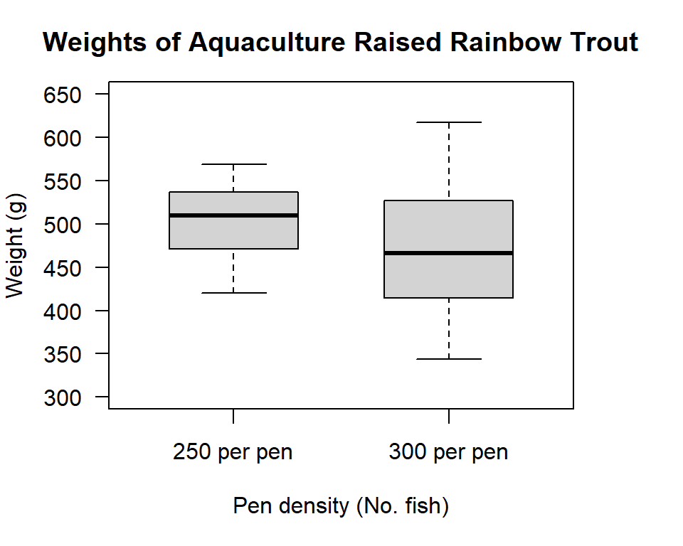
Figure 11.2: Box plot of rainbow trout weight distributions from two aquaculture pen densities (250 fish/pen and 300 fish/pen)
What do you see? It looks like the mean weight is higher for the lower density pen, but the largest fish are from the higher density pen. What about the variances? There looks like less variation in the lower density pen, but does the difference look significant? Let’s see what our test says:
Step 1: Set the Null and Alternate Hypotheses
Null hypothesis: The variance ratio is equal to one
Null hypothesis: The group variances are equal
Alternate hypothesis: The variance ratio is not equal to one
Alternate hypothesis: The group variances are not equal
Step 2: Implement the Variance Ratio Test
Here we provide the data, and two groups separated by a “,” because the data are in wide format. Our alpha value will be set as the default: 0.05.
with(Farmed.Trout, var.test(Trout.250, Trout.300))
#>
#>    F test to compare two variances
#>
#> data:  Trout.250 and Trout.300
#> F = 0.4, num df = 19, denom df = 19, p-value = 0.04
#> alternative hypothesis: true ratio of variances is not equal to 1
#> 95 percent confidence interval:
#>  0.153 0.975
#> sample estimates:
#> ratio of variances
#>              0.386
Step 3: Interpret the Results
From the output we see the p-value = 0.044. Since 0.044 is less than 0.05 (alpha), we: Reject the null hypothesis that the group variances are the same.
What does this mean? It means, we have sufficient evidence to say the variance for fish weight for the two aquaculture pen densities are different.
The variance ratio (0.39) is, in this context, far enough from 1 for us to reject the null.
We also get a 95% confidence interval for the variance ratio of (0.15, 0.97). This range does not include 1. This aligns with the p-value information. If the p-value is less than 0.05 the 95% confidence interval does not contain 1. So, although our 95% upper confidence level is close to 1 our estimate is still quite far away and we reject the null. If we were to move on to test the means of the two groups we would set our t-test parameter
var.equalto FALSE.
11.2 Advanced: Technical Note
Recall that the ratio of sample variances follows an \(F\)-distribution when the variable of interest is normally distributed in each of the populations. The \(F\)-test for equal variances is only valid when this is true and in fact this test is quite sensitive to departures from normality.
Whether or not a variance ratio test should ever be conducted is an open question. Simulation studies have shown that for many cases where the standard t-test performs poorly, and hence we want to use the unequal variance t-test formula, the variance ratio test does not have good ability to accurately determine that the variances of the two groups are different. Conversely, for scenarios where the variance ratio test has good ability to accurately determine that the variance of the two groups are different, just using the standard t-test that incorrectly assumes the variances of the groups are equal still works very well. Combined these two results have led some to conclude that it is better to not ever use a variance ratio test.
To more fully understand the issues involved requires an understanding of what is meant by a type I error; what is meant by the expression power of the test; and the definitions of both the chi-square distribution and the F-distribution. Consideration of such issues is something that is only relevant for students in their 4th or 5th year at university. A relatively accessible reference for such students is provided below. If you are taking an introductory class, these issues are likely to be beyond the scope of the course and before you undertake a two sample t-test you are expected to conduct a variance ratio test.
Reference
Markowski, C. A., & Markowski, E. P. (1990). Conditions for the effectiveness of a preliminary test of variance. The American Statistician}, 44(4), 322-326. https://www.jstor.org/stable/2684360