Chapter 13 Advanced: Technical Details on Two-Sample t-test
In this section we consider a difference in two population means, \(\mu_1 - \mu_2\), under the condition that the data are not paired. Just as with a single sample, we identify conditions to ensure we can use the \(t\)-distribution with a point estimate of the difference, \(\bar{x}_1 - \bar{x}_2\).
We apply these methods in three contexts: determining whether stem cells can improve heart function, exploring the impact of pregnant women’s smoking habits on birth weights of newborns, and exploring whether there is statistically significant evidence that one variations of an exam is harder than another variation. This section is motivated by questions like ``Is there convincing evidence that newborns from mothers who smoke have a different average birth weight than newborns from mothers who don’t smoke?’’
13.1 Confidence interval for a difference of means
Does treatment using embryonic stem cells (ESCs) help improve heart function following a heart attack? Table (13.1) contains summary statistics for an experiment to test ESCs in sheep that had a heart attack. Each of these sheep was randomly assigned to the ESC or control group, and the change in their hearts’ pumping capacity was measured in the study. A positive value corresponds to increased pumping capacity, which generally suggests a stronger recovery. Our goal will be to identify a 95% confidence interval for the effect of ESCs on the change in heart pumping capacity relative to the control group.
A point estimate of the difference in the heart pumping variable can be found using the difference in the sample means:
\[ \bar{x}_{esc} - \bar{x}_{control}\ =\ 3.50 - (-4.33)\ =\ 7.83\]
| \(n\) | \(\bar{x}\) | \(s\) | |
|---|---|---|---|
| ESCs | 9 | 3.50 | 5.17 |
| control | 9 | -4.33 | 2.76 |
We first setup the hypotheses:
- Null hypothesis: The stem cells do not improve heart pumping function. \(\mu_{esc} - \mu_{control} = 0\).
- Alternate hypothesis: The stem cells do improve heart pumping function. \(\mu_{esc} - \mu_{control} > 0\).
Example 13.2 Can the \(t\)-distribution be used to make inference using the point estimate, \(\bar{x}_{esc} - \bar{x}_{control} = 7.83\)?
We check the two required conditions:
- In this study, the sheep were independent of each other. Additionally, the distributions in Figure 13.1 don’t show any clear deviations from normality, where we watch for prominent outliers in particular for such small samples. These findings imply each sample mean could itself be modelled using a \(t\)-distribution.
- The sheep in each group were also independent of each other.
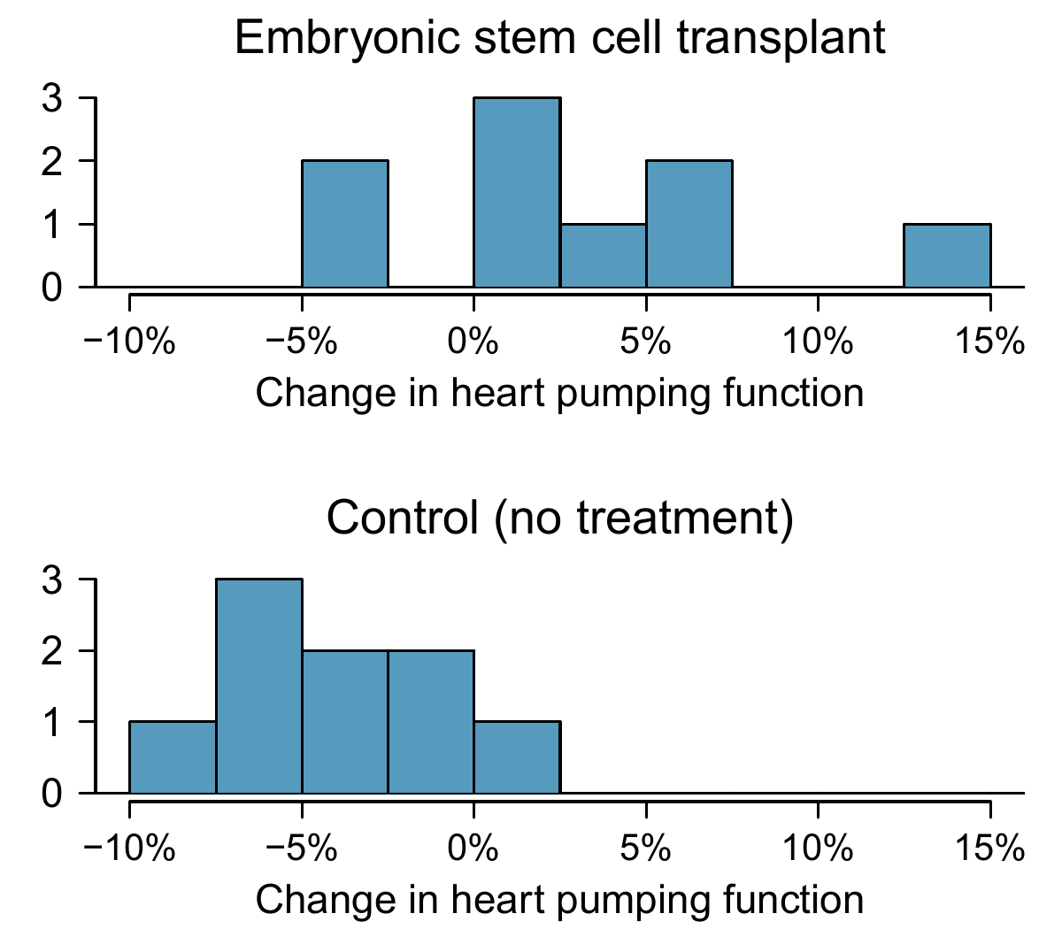
Figure 13.1: Histograms for both the embryonic stem cell group and the control group. Higher values are associated with greater improvement. We don’t see any evidence of skew in these data; however, it is worth noting that skew would be difficult to detect with such a small sample.
When not assuming that the variances are equal, we can quantify the variability in the point estimate, \(\bar{x}_{esc} - \bar{x}_{control}\), using the following formula for its standard error: \[ SE_{\bar{x}_{esc} - \bar{x}_{control}} = \sqrt{\frac{\sigma_{esc}^2}{n_{esc}} + \frac{\sigma_{control}^2}{n_{control}}}\] We usually estimate this standard error using standard deviation estimates based on the samples:
\[\begin{align} SE_{\bar{x}_{esc} - \bar{x}_{control}} &= \sqrt{\frac{\sigma_{esc}^2}{n_{esc}} + \frac{\sigma_{control}^2}{n_{control}}} \\ &\approx \sqrt{\frac{s_{esc}^2}{n_{esc}} + \frac{s_{control}^2}{n_{control}}} \\ &= \sqrt{\frac{5.17^2}{9} + \frac{2.76^2}{9}} = 1.95 \end{align}\]
Because we will use the \(t\)-distribution, we also must identify the appropriate degrees of freedom. This can be done using computer software. An alternative technique is to use the smaller of \(n_1 - 1\) and \(n_2 - 1\), which is the method we will typically apply in the examples and guided practice.120
Example 13.3 Calculate a 95% confidence interval for the effect of ESCs on the change in heart pumping capacity of sheep after they have suffered a heart attack.
We will use the sample difference and the standard error for that point estimate from our earlier calculations:
\[\begin{align*} & \bar{x}_{esc} - \bar{x}_{control} = 7.83 \\ & SE = \sqrt{\frac{5.17^2}{9} + \frac{2.76^2}{9}} = 1.95 \end{align*}\]
Using \(df = 8\), we can identify the appropriate \(t^{\star}_{df} = t^{\star}_{8}\) for a 95% confidence interval as 2.31. Finally, we can enter the values into the confidence interval formula:
\[\begin{align*} \text{point estimate} \ \pm\ t^{\star}SE \quad\rightarrow\quad 7.83 \ \pm\ 2.31\times 1.95 \quad\rightarrow\quad (3.32, 12.34) \end{align*}\]
We are 95% confident that embryonic stem cells improve the heart’s pumping function in sheep that have suffered a heart attack by 3.32% to 12.34%.13.2 Hypothesis tests based on a difference in means
A data set called baby_smoke represents a random sample of 150 cases of mothers and their newborns in North Carolina over a year. Four cases from this data set are represented in Table 13.2. We are particularly interested in two variables: \(\texttt{weight}\) and \(\texttt{smoke}\). The \(\texttt{weight}\) variable represents the weights of the newborns and the \(\texttt{smoke}\) variable describes which mothers smoked during pregnancy. We would like to know, is there convincing evidence that newborns from mothers who smoke have a different average birth weight than newborns from mothers who don’t smoke? We will use the North Carolina sample to try to answer this question. The smoking group includes 50 cases and the nonsmoking group contains 100 cases, represented in Figure 13.2.
| fAge | mAge | weeks | weight | sexBaby | smoke | |
|---|---|---|---|---|---|---|
| 1 | NA | 13 | 37 | 5.00 | female | nonsmoker |
| 2 | NA | 14 | 36 | 5.88 | female | nonsmoker |
| 3 | 19 | 15 | 41 | 8.13 | male | smoker |
| \(\vdots\) | \(\vdots\) | \(\vdots\) | \(\vdots\) | \(\vdots\) | \(\vdots\) | |
| 150 | 45 | 50 | 36 | 9.25 | female | nonsmoker |
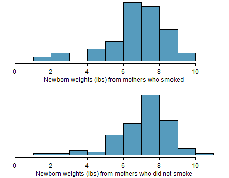
Figure 13.2: The top panel represents birth weights for infants whose mothers smoked. The bottom panel represents the birth weights for infants whose mothers who did not smoke. The distributions exhibit moderate-to-strong and strong~skew, respectively.
Example 13.4 Set up appropriate hypotheses to evaluate whether there is a relationship between a mother smoking and average birth weight.
The null hypothesis represents the case of no difference between the groups.
- Null hypothesis: There is no difference in average birth weight for newborns from mothers who did and did not smoke. In statistical notation: \(\mu_{n} - \mu_{s} = 0\), where \(\mu_{n}\) represents non-smoking mothers and \(\mu_s\) represents mothers who smoked.
- Alternate hypothesis: There is some difference in average newborn weights from mothers who did and did not smoke (\(\mu_{n} - \mu_{s} \neq 0\)).
We check the two conditions necessary to apply the \(t\)-distribution to the difference in sample means. (1) Because the data come from a simple random sample and consist of less than 10% of all such cases, the observations are independent. Additionally, while each distribution is strongly skewed, the sample sizes of 50 and 100 would make it reasonable to model each mean separately using a \(t\)-distribution. The skew is reasonable for these sample sizes of 50 and 100. (2) The independence reasoning applied in (1) also ensures the observations in each sample are independent. Since both conditions are satisfied, the difference in sample means may be modelled using a \(t\)-distribution.
Summary statistics are shown for each sample in Table 13.3.
| fAge | smoker | nonsmoker |
|---|---|---|
| mean | 6.78 | 7.18 |
| standard deviation | 1.43 | 1.60 |
| sample size | 50 | 100 |
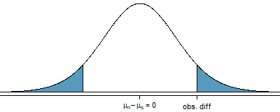
Example 13.5 Draw a picture to represent the p-value for the hypothesis test from Example 13.4.
To depict the p-value, we draw the distribution of the point estimate as though \(H_0\) were true and shade areas representing at least as much evidence against \(H_0\) as what was observed. Both tails are shaded because it is a two-sided test.
Example 13.6 Compute the p-value of the hypothesis test using the figure in Example 13.5, and evaluate the hypotheses using a significance level of \(\alpha=0.05\).
We start by computing the T-score: \[\begin{eqnarray*} T = \frac{\ 0.40 - 0\ }{0.26} = 1.54 \end{eqnarray*}\]Next, we compare this value to values in the \(t\)-table which can be found online, for example http://www.ttable.org/. Alternatively, this probability can be found using R. We use the pt() function to find the probability to the right of 1.54 in the \(t\)-distribution, we then double this probability to get the two-sided probability.We use the smaller of \(n_n - 1 = 99\) and \(n_s - 1 = 49\) as the degrees of freedom: \(df = 49\).
2*pt(q = 1.54 , df = 49, lower.tail = FALSE)
#> [1] 0.13
This p-value is larger than the significance value, 0.05, so we fail to reject the null hypothesis. There is insufficient evidence to say there is a difference in average birth weight of newborns from North Carolina mothers who did smoke during pregnancy and newborns from North Carolina mothers who did not smoke during pregnancy.
Public service announcement: while we have used this relatively small data set as an example, larger data sets show that women who smoke tend to have smaller newborns. In fact, some in the tobacco industry actually had the audacity to tout that as a benefit of smoking:
It’s true. The babies born from women who smoke are smaller, but they’re just as healthy as the babies born from women who do not smoke. And some women would prefer having smaller babies.- Joseph Cullman, Philip Morris’ Chairman of the Board on CBS’ Face the Nation, Jan 3, 1971
Fact check: the babies from women who smoke are not actually as healthy as the babies from women who do not smoke.124
Case study: two versions of a course exam
An instructor decided to run two slight variations of the same exam. Prior to passing out the exams, she shuffled the exams together to ensure each student received a random version. Summary statistics for how students performed on these two exams are shown in Table 13.4. Anticipating complaints from students who took Version B, she would like to evaluate whether the difference observed in the groups is so large that it provides convincing evidence that Version B was more difficult (on average) than Version A.
| Version | \(n\) | \(\bar{x}\) | \(s\) | min | max |
|---|---|---|---|---|---|
| A | 30 | 79.4 | 14 | 45 | 100 |
| B | 27 | 74.1 | 20 | 32 | 100 |
After verifying the conditions for each sample and confirming the samples are independent of each other, we are ready to conduct the test using the \(t\)-distribution. In this case, we are estimating the true difference in average test scores using the sample data, so the point estimate is \(\bar{x}_A - \bar{x}_B = 5.3\). The standard error of the estimate can be calculated as
\[\begin{eqnarray*} SE = \sqrt{\frac{s_A^2}{n_A} + \frac{s_B^2}{n_B}} = \sqrt{\frac{14^2}{30} + \frac{20^2}{27}} = 4.62 \end{eqnarray*}\] Finally, we construct the test statistic: \[\begin{eqnarray*} T = \frac{\text{point estimate} - \text{null value}}{SE} = \frac{(79.4-74.1) - 0}{4.62} = 1.15 \end{eqnarray*}\]
If we have a computer handy, we can identify the degrees of freedom as 45.97. Otherwise we use the smaller of \(n_1-1\) and \(n_2-1\): \(df=26\).
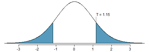
Figure 13.3: The \(t\)-distribution with 26 degrees of freedom. The shaded right tail represents values with \(T >= 1.15\). Because it is a two-sided test, we also shade the corresponding lower tail.
Example 13.7 Identify the p-value using \(df = 26\) and provide a conclusion in the context of the case study.
We examine row \(df=26\) in the \(t\)-table. Because this value is smaller than the value in the left column, the p-value is larger than 0.200 (two tails!). Because the p-value is so large, we do not reject the null hypothesis. That is, the data do not convincingly show that one exam version is more difficult than the other, and the teacher should not be convinced that she should add points to the Version B exam scores.13.3 Summary for inference using the \(t\)-distribution
When considering the difference of two means, there are two common cases: the two samples are paired or they are independent. (There are instances where the data are neither paired nor independent, e.g. blocking in designed experiments) The paired case was treated in Section 14, where the one-sample methods were applied to the differences from the paired observations. We examined the second and more complex scenario in this section.
Hypothesis tests. When applying the \(t\)-distribution for a hypothesis test, we proceed as follows:
- Write appropriate hypotheses.
- Verify conditions for using the \(t\)-distribution.
- One-sample or differences from paired data: the observations (or differences) must be independent and nearly normal. For larger sample sizes, we can relax the nearly normal requirement, e.g. slight skew is okay for sample sizes of 15, moderate skew for sample sizes of 30, and strong skew for sample sizes of 60.
- For a difference of means when the data are not paired: each sample mean must separately satisfy the one-sample conditions for the \(t\)-distribution, and the data in the groups must also be independent.
- Compute the point estimate of interest, the standard error, and the degrees of freedom. For \(df\), use \(n-1\) for one sample, and for two samples use either statistical software or the smaller of \(n_1 - 1\) and \(n_2 - 1\).
- Compute the T-score and p-value.
- Make a conclusion based on the p-value, and write a conclusion in context and in plain language so anyone can understand the result.
Confidence intervals. Similarly, the following is how we generally computed a confidence interval using a \(t\)-distribution:
- Verify conditions for using the \(t\)-distribution. (See above.)
- Compute the point estimate of interest, the standard error, the degrees of freedom, and \(t^{\star}_{df}\).
- Calculate the confidence interval using the general formula, point estimate \(\pm\ t_{df}^{\star} SE\).
- Put the conclusions in context and in plain language so even non-statisticians can understand the results.
13.4 Examining the standard error formula (special topic)
The formula for the standard error of the difference in two means is similar to the formula for other standard errors. Recall that the standard error of a single mean, \(\bar{x}_1\), can be approximated by
\[\begin{align*} SE_{\bar{x}_1} = \frac{s_1}{\ \sqrt{n_1}\ } \end{align*}\] where \(s_1\) and \(n_1\) represent the sample standard deviation and sample size.
The standard error of the difference of two sample means can be constructed from the standard errors of the separate sample means: \[\begin{align} SE_{\bar{x}_{1} - \bar{x}_{2}} &= \sqrt{SE_{\bar{x}_1}^2 + SE_{\bar{x}_2}^2}\\ &= \sqrt{\frac{s_1^2}{{n_1}} + \frac{s_2^2}{{n_2}}} \tag{13.2} \end{align}\] This special relationship follows from probability theory.
13.5 Pooled standard deviation estimate (special topic)
Occasionally, two populations will have standard deviations that are so similar that they can be treated as identical. For example, historical data or a well-understood biological mechanism may justify this strong assumption. In such cases, we can make the \(t\)-distribution approach slightly more precise by using a pooled standard deviation.
The pooled standard deviation of two groups is a way to use data from both samples to better estimate the standard deviation and standard error. If \(s_1^{}\) and \(s_2^{}\) are the standard deviations of groups 1 and 2 and there are good reasons to believe that the population standard deviations are equal, then we can obtain an improved estimate of the group variances by pooling their data:
\[\begin{align*} s_{pooled}^2 = \frac{s_1^2\times (n_1-1) + s_2^2\times (n_2-1)}{n_1 + n_2 - 2} \end{align*}\] where \(n_1\) and \(n_2\) are the sample sizes, as before. To use this new statistic, we substitute \(s_{pooled}^2\) in place of \(s_1^2\) and \(s_2^2\) in the standard error formula, and we use an updated formula for the degrees of freedom: \[\begin{align*} df = n_1 + n_2 - 2 \end{align*}\]
The benefits of pooling the standard deviation are realized through obtaining a better estimate of the standard deviation for each group and using a larger degrees of freedom parameter for the \(t\)-distribution. Both of these changes may permit a more accurate model of the sampling distribution of \(\bar{x}_1 - \bar{x}_2\), if the standard deviations of the two groups are equal.
Caution Pool standard deviations only after careful consideration
A pooled standard deviation is used when a variance ratio test indicates it is appropriate. When the sample size is large and the condition may be adequately checked with data, the benefits of pooling the standard deviations greatly diminishes.
This technique for degrees of freedom is conservative with respect to a Type 1 Error; it is more difficult to reject the null hypothesis using this \(df\) method. In this example, computer software would have provided us a more precise degrees of freedom of \(df = 12.225\).↩︎
(a) The difference in sample means is an appropriate point estimate: \(\bar{x}_{n} - \bar{x}_{s} = 0.40\). (b) The standard error of the estimate can be estimated using Equation (13.1): \[\begin{eqnarray*} SE = \sqrt{\frac{\sigma_n^2}{n_n} + \frac{\sigma_s^2}{n_s}} \approx \sqrt{\frac{s_n^2}{n_n} + \frac{s_s^2}{n_s}} = \sqrt{\frac{1.60^2}{100} + \frac{1.43^2}{50}} = 0.26 \end{eqnarray*}\]↩︎
Absolutely not. It is possible that there is some difference but we did not detect it. If there is a difference, we made a Type 2 Error. Notice: we also don’t have enough information to, if there is an actual difference, confidently say which direction that difference would be in.↩︎
We could have collected more data. If the sample sizes are larger, we tend to have a better shot at finding a difference if one exists.↩︎
You can watch an episode of John Oliver on Last Week Tonight to explore the present day offenses of the tobacco industry. Please be aware that there is some adult language: www.youtu.be/6UsHHOCH4q8 .↩︎
Because the teacher did not expect one exam to be more difficult prior to examining the test results, she should use a two-sided hypothesis test. \(H_0\): the exams are equally difficult, on average. \(\mu_A - \mu_B = 0\). \(H_A\): one exam was more difficult than the other, on average. \(\mu_A - \mu_B \neq 0\).↩︎
(a) It is probably reasonable to conclude the scores are independent, provided there was no cheating. (b) The summary statistics suggest the data are roughly symmetric about the mean, and it doesn’t seem unreasonable to suggest the data might be normal. Note that since these samples are each nearing 30, moderate skew in the data would be acceptable. (c) It seems reasonable to suppose that the samples are independent since the exams were handed out randomly.↩︎
The standard error squared represents the variance of the estimate. If \(X\) and \(Y\) are two random variables with variances \(\sigma_x^2\) and \(\sigma_y^2\), then the variance of \(X-Y\) is \(\sigma_x^2 + \sigma_y^2\). Likewise, the variance corresponding to \(\bar{x}_1 - \bar{x}_2\) is \(\sigma_{\bar{x}_1}^2 + \sigma_{\bar{x}_2}^2\). Because \(\sigma_{\bar{x}_1}^2\) and \(\sigma_{\bar{x}_2}^2\) are just another way of writing \(SE_{\bar{x}_1}^2\) and \(SE_{\bar{x}_2}^2\), the variance associated with \(\bar{x}_1 - \bar{x}_2\) may be written as \(SE_{\bar{x}_1}^2 + SE_{\bar{x}_2}^2\).↩︎