Chapter 7 Probability

Probability forms a foundation for statistics. You might already be familiar with many aspects of probability, however, formalization of the concepts is new for most. This chapter aims to introduce probability on familiar terms using processes most people have seen before.

7.1 Defining Probability

Guided Practice7.1 A “die,” the singular of dice, is a cube with six faces numbered $1,2,3,4,5$ and $6$. What is the chance of getting $1$ when rolling a die?¹⁰

Guided Practice7.2 What is the chance of getting a $1$ or $2$ in the next roll?¹¹

Guided Practice7.3 What is the chance of getting either $1,2,3,4,5$ or $6$ on the next roll?¹²

Guided Practice7.4 What is the chance of not rolling a $2$?¹³

Guided Practice7.5 Consider rolling two dice. If $1/6^{th}$ of the time the first die is a $1$ and $1/6^{th}$ of those times the second die is a $1$, what is the chance of getting two $1$s?¹⁴

Probability

We use probability to build tools to describe and understand apparent randomness. We often frame probability in terms of a random process giving rise to an outcome.

Action	$\rightarrow$	Outcome
Roll a die	$\rightarrow$	$1,2,3,4,5$ or $6$
Flip a coin	$\rightarrow$	$H$ or $T$

Rolling a die or flipping a coin is a seemingly random process and each gives rise to an outcome.

Definition 7.1 (Probability) The probability of an outcome is the proportion of times the outcome would occur if we observed the random process an infinite number of times.

Probability is defined as a proportion, and it always takes values between 0 and 1 (inclusively). It may also be displayed as a percentage between 0% and 100%.

Probability can be illustrated by rolling a die many times. Let $\hat{p}_n$ be the proportion of outcomes that are $1$ after the first $n$ rolls. As the number of rolls increases, $\hat{p}_n$ will converge to the probability of rolling a $1$, $p = 1/6$. Figure 7.1 shows this convergence for 100,000 die rolls. The tendency of $\hat{p}_n$ to stabilize around $p$ is described by the Law of Large Numbers.

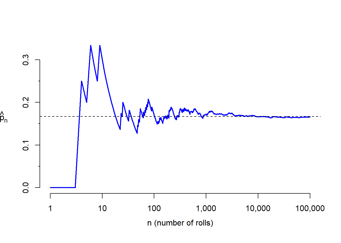
$The fraction of die rolls that are 1 at each stage in a simulation. The proportion tends to get closer to the probability $1/6 \approx 0.167$ as the number of rolls increases.$

Figure 7.1: The fraction of die rolls that are 1 at each stage in a simulation. The proportion tends to get closer to the probability $1/6 \approx 0.167$ as the number of rolls increases.

Definition 7.2 (Law of Large Numbers) As more observations are collected, the proportion $\hat{p}_n$ of occurrences with a particular outcome converges to the probability $p$ of that outcome.

Occasionally the proportion will veer off from the probability and appear to defy the Law of Large Numbers, as $\hat{p}_n$ does many times in Figure 7.1. However, these deviations become smaller as the number of rolls increases.

Above we write $p$ as the probability of rolling a $4$. We can also write this probability as \[P(\textrm{ rolling a }1 \textrm{ })\]

As we become more comfortable with this notation, we will abbreviate it further. For instance, if it is clear that the process is “rolling a die,” we could abbreviate $P(\textrm{ rolling a }1)$ as $P(1)$.

Guided Practice7.6 Random processes include rolling a die and flipping a coin.

Think of another random process.
Describe all the possible outcomes of that process.

For instance, rolling a die is a random process with possible outcomes $1,2,\ldots,6$.¹⁵

Disjoint or mutually exclusive outcomes

Two outcomes are called disjoint or mutually exclusive if they cannot both happen. For instance, if we roll a die, the outcomes $1$ and $2$ are disjoint since they cannot both occur. On the other hand, the outcomes $1$ and “rolling an odd number” are not disjoint since both occur if the outcome of the roll is a $1$. The terms disjoint and mutually exclusive are equivalent and interchangeable.

Calculating the probability of disjoint outcomes is easy. When rolling a die, the outcomes $1$ and $2$ are disjoint, and we compute the probability that one of these outcomes will occur by adding their separate probabilities:

\[ P(1\textrm{ or }2) = P(1)+P(2) = 1/6 + 1/6 = 1/3 \]

What about the probability of rolling a $1,2,3,4,5$ or $6$? Here again, all of the outcomes are disjoint so we add the probabilities:

\[ \begin{aligned} &P(1 \textrm{ or } 2 \textrm{ or } 3 \textrm{ or } 4 \textrm{ or } 5 \textrm{ or } 6)\\ &\quad= P(1)+P(2)+P(3)+P(4)+P(5)+P(6)\\ &\quad= 1/6 + 1/6 + 1/6 + 1/6 + 1/6 + 1/6 = 1. \end{aligned} \]

The Addition Rule guarantees the accuracy of this approach when the outcomes are disjoint.

Definition 7.3 (Addition Rule of disjoint outcomes) If $A_1$ and $A_2$ represent two disjoint outcomes, then the probability that one of them occurs is given by

\[P(A_1\textrm{ or } A_2) = P(A_1) + P(A_2)\]

If there are many disjoint outcomes $A_1,\ldots ,A_k$, then the probability that one of these outcomes will occur is

\[P(A_1) + P(A_2) + \cdots + P(A_k)\]

Guided Practice7.7 We are interested in the probability of rolling a $1, 4,$$5$. (a) Explain why the outcomes $1$, $4$, and $5$ are disjoint. (b) Apply the Addition Rule for disjoint outcomes (Definition 7.3) to determine $P(1\textrm{ or }4\textrm{ or }5)$.¹⁶

Guided Practice7.8 Load and inspect the email data set as follows.

install.packages("openintro") #install the package containing the data
library(openintro) #load the package that contains the data
help("email") # inspect the help file describing the data
head(email) # inspect the first few rows of the data

The number variable described whether no number (labeled none), only one or more small numbers (small), or whether at least one big number appeared in an email (big).

length(email$number)
#> [1] 3921
table(email$number)
#> 
#>  none small   big 
#>   549  2827   545

Of the 3,921 emails, 549 had no numbers, 2,827 had only one or more small numbers, and 545 had at least one big number. (a) Are the outcomes none, small, and big disjoint? (b) Determine the proportion of emails with value small and big separately. (c) Use the Addition Rule for disjoint outcomes to compute the probability a randomly selected email from the data set has a number in it, small or big.¹⁷

Statisticians rarely work with individual outcomes and instead consider sets or collections of outcomes. Let $A$ represent the event where a die roll results in $1$ or $2$ and $B$~represent the event that the die roll is a $4$ or a $6$. We write $A$ as the set of outcomes $\{1,2\}$ and $B=\{4,6\}$. These sets are commonly called event. Because $A$ and $B$ have no elements in common, they are disjoint events. $A$ and $B$ are represented in Figure 7.2.

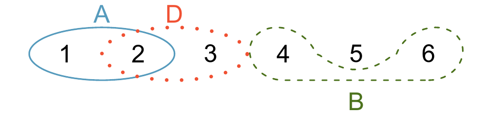
Figure 7.2: Three events, $A$, $B$, and $D$, consist of outcomes from rolling a die. $A$ and $B$ are disjoint since they do not have any outcomes in common.

The Addition Rule applies to both disjoint outcomes and disjoint events. The probability that one of the disjoint events $A$ or $B$ occurs is the sum of the separate probabilities: \[ P(A\text{ or }B) = P(A) + P(B) = 1/3 + 1/3 = 2/3 \]

Guided Practice7.9 (a) Verify the probability of event $A$, $P(A)$, is $1/3$ using the Addition Rule. (b) Do the same for event $B$.

Guided Practice7.10 (a) Using Figure 7.2 as a reference, what outcomes are represented by event $D$? (b) Are events $B$ and $D$ disjoint? (c) Are events $A$ and $D$ disjoint?¹⁸

Guided Practice7.11 In Guided Practice 7.10, you confirmed $B$ and $D$ from Figure 7.2 are disjoint. Compute the probability that event $B$ or event $D$ occurs.¹⁹.

7.1.1 Probabilities when events are not disjoint

Let’s consider calculations for two events that are not disjoint in the context of a regular deck of 52 cards, represented in Table 7.1. If you are unfamiliar with the cards in a regular deck, please see the footnote²⁰.

Table 7.1: Representations of the 52 unique cards in a deck.
$2\clubsuit$	$3\clubsuit$	$4\clubsuit$	$5\clubsuit$	$6\clubsuit$	$7\clubsuit$	$8\clubsuit$	$9\clubsuit$	$10\clubsuit$	$J\clubsuit$	$Q\clubsuit$	$K\clubsuit$	$A\clubsuit$
$\color{red}{2\diamondsuit}$	$\color{red}{3\diamondsuit}$	$\color{red}{4\diamondsuit}$	$\color{red}{5\diamondsuit}$	$\color{red}{6\diamondsuit}$	$\color{red}{7\diamondsuit}$	$\color{red}{8\diamondsuit}$	$\color{red}{9\diamondsuit}$	$\color{red}{10\diamondsuit}$	$\color{red}{J\diamondsuit}$	$\color{red}{Q\diamondsuit}$	$\color{red}{K\diamondsuit}$	$\color{red}{A\diamondsuit}$
$\color{red}{2\heartsuit}$	$\color{red}{3\heartsuit}$	$\color{red}{4\heartsuit}$	$\color{red}{5\heartsuit}$	$\color{red}{6\heartsuit}$	$\color{red}{7\heartsuit}$	$\color{red}{8\heartsuit}$	$\color{red}{9\heartsuit}$	$\color{red}{10\heartsuit}$	$\color{red}{J\heartsuit}$	$\color{red}{Q\heartsuit}$	$\color{red}{K\heartsuit}$	$\color{red}{A\heartsuit}$
$2\spadesuit$	$3\spadesuit$	$4\spadesuit$	$5\spadesuit$	$6\spadesuit$	$7\spadesuit$	$8\spadesuit$	$9\spadesuit$	$10\spadesuit$	$J\spadesuit$	$Q\spadesuit$	$K\spadesuit$	$A\spadesuit$

Guided Practice7.12 (a) What is the probability that a randomly selected card is a diamond? (b) What is the probability that a randomly selected card is a face card?²¹

Venn diagrams are useful when outcomes can be categorized as “in” or “out” for two or three variables, attributes, or random processes. The Venn diagram in Figure 7.3 uses a circle to represent diamonds and another to represent face cards. If a card is both a diamond and a face card, it falls into the intersection of the circles. If it is a diamond but not a face card, it will be in part of the left circle that is not in the right circle (and so on). The total number of cards that are diamonds is given by the total number of cards in the diamonds circle: $10+3=13$. The probabilities are also shown (e.g. $10/52 = 0.1923$).

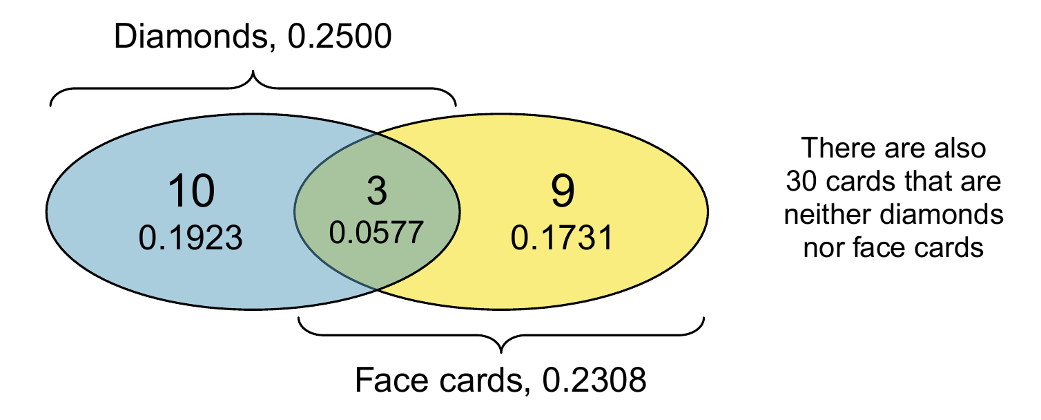
Figure 7.3: A Venn diagram for diamonds and face cards.

Guided Practice7.13 Using Figure 7.3, verify $P(\text{face card}) = 12/52=3/13$.²²

Let $A$ represent the event that a randomly selected card is a diamond and $B$ represent the event that it is a face card. How do we compute $P(A\text{ or }B)$? Events $A$ and $B$ are not disjoint – the cards $\color{red}{J\diamondsuit}$, $\color{red}{Q\diamondsuit}$, and $\color{red}{K\diamondsuit}$ fall into both categories – so we cannot use the Addition Rule for disjoint events. Instead we use the Venn diagram. We start by adding the probabilities of the two events:

\[ \begin{aligned} &P(A) + P(B)\\ &= P({\color{red}\diamondsuit}) + P(\text{face card})\\ &= 13/52 + 12/52 \end{aligned} \tag{7.1} \]

However, the three cards that are in both events were counted twice, once in each probability. We must correct this double counting: \[ \begin{aligned} &P(A\text{ or } B) \\ =&P({\color{red}\diamondsuit}\text{ or face card}) \\ =& P({\color{red}\diamondsuit}) + P(\text{face card}) - P({\color{red}\diamondsuit}\text{ and face card})\\ =& 13/52 + 12/52 - 3/52 \\ =& 22/52 = 11/26 \end{aligned} \tag{7.2} \] Equation (7.2) is an example of the General Addition Rule.

Definition 7.4 (General Addition Rule) If $A$ and $B$ are any two events, disjoint or not, then the probability that at least one of them will occur is

\[ P(A\text{ or }B) = P(A) + P(B) - P(A\text{ and }B) \tag{7.3} \] where $P(A\text{ and }B)$ is the probability that both events occur.

Remark (or is inclusive). When we write “or” in probability and statistics, we mean “and/or” unless we explicitly state otherwise. Thus, $A$ or $B$ occurs means $A$, $B$, or both $A$ and $B$ occur.

Guided Practice7.14
(a) If $A$ and $B$ are disjoint, describe why this implies $P(A \text{ and }B) = 0$.
(b) Using part (a), verify that the General Addition Rule simplifies to the simpler Addition Rule for disjoint events if $A$ and $B$ are disjoint.²³

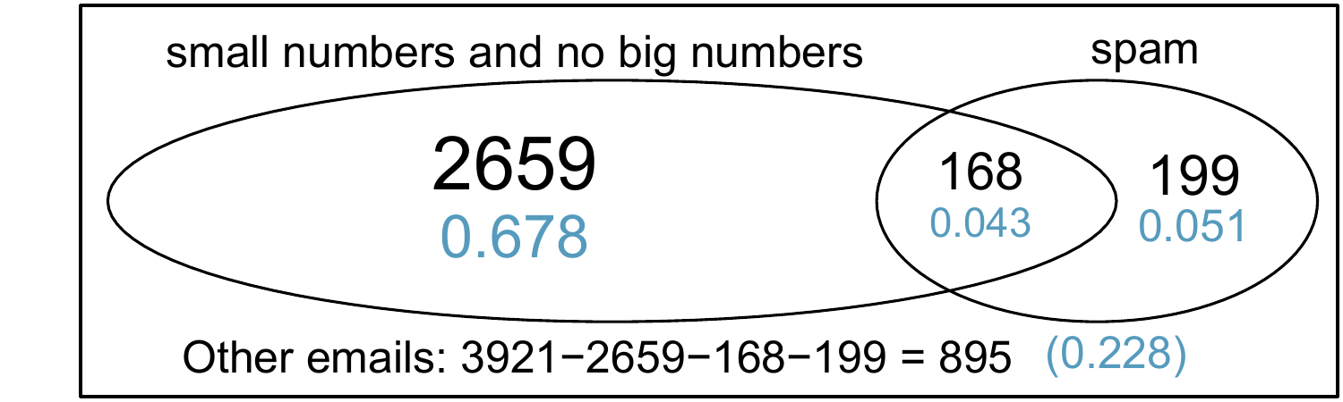
Guided Practice7.15 In the email data set with 3,921 emails, 367 were spam, 2,827 contained some small numbers but no big numbers, and 168 had both characteristics. Create a Venn diagram for this setup.

Solution. Both the counts and corresponding probabilities (e.g. $2659/3921 = 0.678$) are shown. Notice that the number of emails represented in the left circle corresponds to $2659 + 168 = 2827$, and the number represented in the right circle is $168 + 199 = 367$.

Guided Practice7.16
(a) Use your Venn diagram from Guided Practice 7.15 to determine the probability a randomly drawn email from the email data set is spam and had small numbers (but not big numbers).
(b) What is the probability that the email had either of these attributes?²⁴

7.1.2 Probability distributions

A probability distribution is a table of all disjoint outcomes and their associated probabilities. Table 7.2 shows the probability distribution for the sum of two dice.

Table 7.2: Probability distribution for the sum of two dice.
Dice sum	2	3	4	5	6	7	8	9	10	11	12
Probability	$\frac{1}{36}$	$\frac{2}{36}$	$\frac{3}{36}$	$\frac{4}{36}$	$\frac{5}{36}$	$\frac{6}{36}$	$\frac{5}{36}$	$\frac{4}{36}$	$\frac{3}{36}$	$\frac{2}{36}$	$\frac{1}{36}$

Guided Practice7.17 Table 7.3 suggests three distributions for household income in Australia. Only one is correct. Which one must it be? What is wrong with the other two?²⁵

Table 7.3: Proposed distributions of Australian household incomes.
Weekly income range ($1000s)	0-1	1-2	2-3	3-4	4-5	5+
(a)	0.33	0.28	0.19	0.10	0.04	0.05
(b)	0.33	-0.28	0.19	0.10	0.04	0.05
(c)	0.23	0.18	0.19	0.10	0.04	0.05

Probability distributions can be summarized in a bar plot. For instance, the distribution of Australian household incomes²⁶ is shown in Figure 7.4 as a bar plot. The probability distribution for the sum of two dice is shown in Table 7.2 and plotted in Figure 7.5.

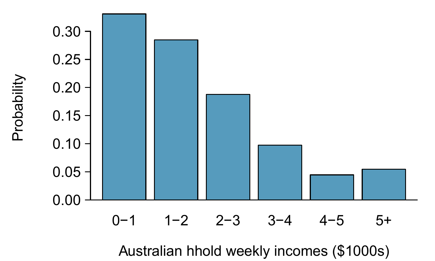
Figure 7.4: The probability distribution of Australian household income.

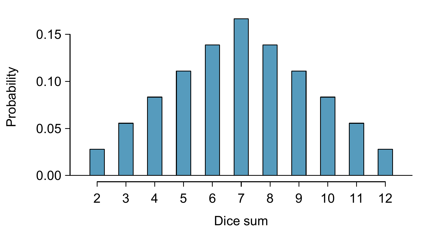
Figure 7.5: The probability distribution of the sum of two dice.

In these bar plots, the bar heights represent the probabilities of outcomes. If the outcomes are numerical and discrete, it is usually (visually) convenient to make a bar plot that resembles a histogram, as in the case of the sum of two dice.

7.1.3 Complement of an event

Rolling a die produces a value in the set $\{1,2,3,4,5,6\}$. This set of all possible outcomes is called the sample space ($S$) for rolling a die. We often use the sample space to examine the scenario where an event does not occur.

Let $D=\{2, 3\}$ represent the event that the outcome of a die roll is $2$ or $3$. Then the complement of $D$ represents all outcomes in our sample space that are not in $D$, which is denoted by $D^c = \{1,4, 5,6\}$. That is, $D^c$ is the set of all possible outcomes not already included in $D$. Figure 7.6 shows the relationship between $D$, $D^c$, and the sample space $S$.

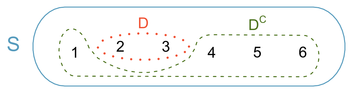
$Event $D=\\{2, 3\\}$ and its complement, $D^c = \\{1, 4, 5, 6\\}$. $S$ represents the sample space, which is the set of all possible events.$

Figure 7.6: Event $D=\\{2, 3\\}$ and its complement, $D^c = \\{1, 4, 5, 6\\}$. $S$ represents the sample space, which is the set of all possible events.

Guided Practice7.18
(a) Compute $P(D^c) = P(\text{rolling a }1, 4, 5,\text{ or } 6)$.
(b) What is $P(D) + P(D^c)$?²⁷

Guided Practice7.19 Events $A=\{1,2\}$ and $B=\{4, 6\}$ are shown in Figure 7.2.

Write out what $A^c$ and $B^c$ represent.
Compute $P(A^c)$ and $P(B^c)$.
Compute $P(A)+P(A^c)$ and $P(B)+P(B^c)$.²⁸

A complement of an event $A$ is constructed to have two very important properties:

every possible outcome not in $A$ is in $A^c$, and
$A$ and $A^c$ are disjoint.

Property (i) implies

\[ P(A\text{ or }A^c) = 1 \tag{7.4} \]

That is, if the outcome is not in $A$, it must be represented in $A^c$. We use the Addition Rule for disjoint events to apply Property (ii): \[ P(A\text{ or }A^c) = P(A) + P(A^c) \tag{7.5} \] Combining Equations @ref(eq:complementSumTo1 and (7.5) yields a very useful relationship between the probability of an event and its complement.

Definition 7.5 (Complement) The complement of event $A$ is denoted $A^c$, and $A^c$ represents all outcomes not in~$A$. $A$ and $A^c$ are mathematically related: \[ P(A) + P(A^c) = 1, \quad\text{i.e.}\quad P(A) = 1-P(A^c) \tag{7.6} \]

In simple examples, computing $A$ or $A^c$ is feasible in a few steps. However, using the complement can save a lot of time as problems grow in complexity.

Guided Practice7.20 Let $A$ represent the event where we roll two dice and their total is less than $12$.
(a) What does the event $A^c$ represent?
(b) Determine $P(A^c)$ from Table 7.2.
(c) Determine $P(A)$.²⁹

Guided Practice7.21 Consider again the probabilities from Table 7.2 and rolling two dice. Find the following probabilities:
(a) The sum of the dice is not $6$.
(b) The sum is at least $4$. That is, determine the probability of the event $B=\{4, 5,\ldots ,12\}$.
(c) The sum is no more than $10$. That is, determine the probability of the event $D=\{2, 3, \ldots ,10\}$.³⁰

7.1.4 Independence

Just as variables and observations can be independent, random processes can be independent, too. Two processes are independent if knowing the outcome of one provides no useful information about the outcome of the other. For instance, flipping a coin and rolling a die are two independent processes – knowing the coin was heads does not help determine the outcome of a die roll. On the other hand, stock prices usually move up or down together, so they are not independent.

Example 7.5 provides a basic example of two independent processes: rolling two dice. We want to determine the probability that both will be $1$. Suppose one of the dice is red and the other white. If the outcome of the red die is a $1$, it provides no information about the outcome of the white die. We first encountered this same question in Example 7.5, where we calculated the probability using the following reasoning: $1/6^{th}$ of the time the red die is a $1$, and $1/6^{th}$ of those times the white die will also be $1$. This is illustrated in Figure 7.7. Because the rolls are independent, the probabilities of the corresponding outcomes can be multiplied to get the final answer: $(1/6)\times(1/6)=1/36$. This can be generalized to many independent processes.

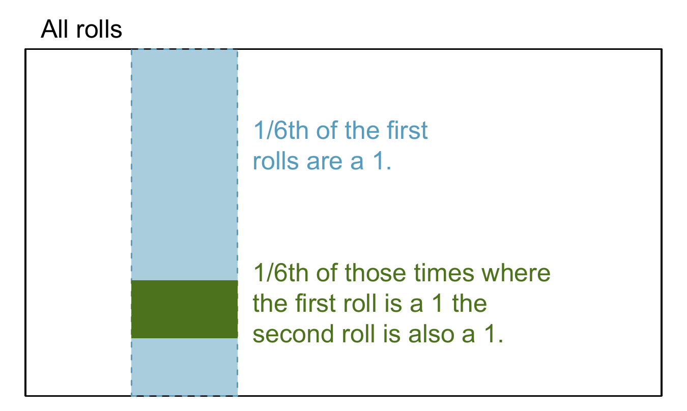
$$1/6^{th}$ of the time, the first roll is a $1$. Then $1/6^{th}$ of those times, the second roll will also be a $1$.$

Figure 7.7: $1/6^{th}$ of the time, the first roll is a $1$. Then $1/6^{th}$ of those times, the second roll will also be a $1$.

Example 7.1 What if there was also a blue die independent of the other two? What is the probability of rolling the three dice and getting all $1$s?

The same logic applies from Example 7.5. If $1/36^{th}$ of the time the white and red dice are both $1$, then $1/6^{th}$ of those times the blue die will also be $1$, so multiply:

\[ \begin{aligned} &P(\texttt{white}=1 \text{ and } \texttt{red}=1 \text{ and }\texttt{blue}=1)\\ &= P(\texttt{white}=1)\times P(\texttt{red}=1)\times P(\texttt{blue}=1) \\ &= (1/6)\times (1/6)\times (1/6)\\ &= 1/216 \end{aligned} \]

Example 7.1 illustrates what is called the Multiplication Rule for independent processes.

Definition 7.6 (Multiplication Rule for independent processes) If $A$ and $B$ represent events from two different and independent processes, then the probability that both $A$ and $B$ occur can be calculated as the product of their separate probabilities:

\[ P(A \text{ and }B) = P(A) \times P(B) \tag{7.7} \] Similarly, if there are $k$ events $A_1$, …, $A_k$ from $k$ independent processes, then the probability they all occur is \[ P(A_1) \times P(A_2)\times \cdots \times P(A_k) \]

Sometimes we wonder if one outcome provides useful information about another outcome. The question we are asking is, are the occurrences of the two events independent? We say that two events $A$ and $B$ are independent if they satisfy Equation (7.7).

Example 7.2 If we shuffle up a deck of cards and draw one, is the event that the card is a heart independent of the event that the card is an ace?

The probability the card is a heart is $1/4$ and the probability that it is an ace is $1/13$. The probability the card is the ace of hearts is $1/52$. We check whether Equation (7.7) is satisfied:

\[ \begin{aligned} P({\color{red}\heartsuit})\times P(\text{ace}) &= \frac{1}{4}\times \frac{1}{13} \\ &= \frac{1}{52} \\ &= P({\color{red}\heartsuit}\text{ and ace}) \end{aligned} \]

Because the equation holds, the event that the card is a heart and the event that the card is an ace are independent events.

7.2 Conditional Probability

The family_college data set contains a sample of 792 cases with two variables, $\texttt{teen}$ and $\texttt{parents}$, and is summarized in Table 7.4.³¹ The $\texttt{teen}$ variable is either $\texttt{college}$ or $\texttt{not}$, where the $college$ label means the teen went to college immediately after high school. The $\texttt{parents}$ variable takes the value $\texttt{degree}$ if at least one parent of the teenager completed a college degree.

Table 7.4: Contingency table summarizing the `family_college` data set.
	parents
	degree	not	Total
college	231	214	445
not	49	298	347
Total	280	512	792

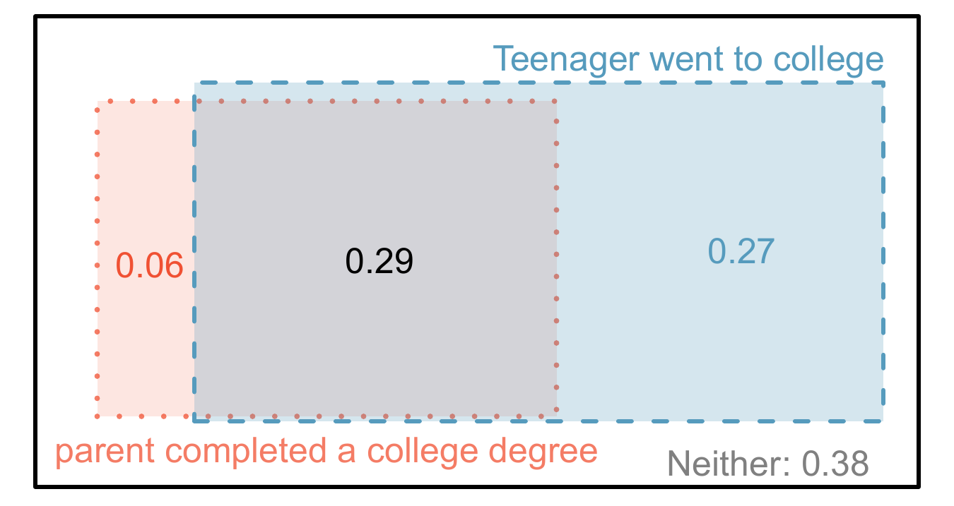
Figure 7.8: A Venn diagram using boxes for the family_college data set.

Example 7.3 If at least one parent of a teenager completed a college degree, what is the chance the teenager attended college right after high school?

We can estimate this probability using the data. Of the 280 cases in this data set where $parents$ takes value $degree$, 231 represent cases where the $teen$ variable takes value $college$:

\[ \begin{aligned} &P(\texttt{teen}=\texttt{college} \text{ given }\texttt{parents}=\texttt{degree}) \\ &= \frac{231}{280} \\ &= 0.825 \end{aligned} \]

Example 7.4 A teenager is randomly selected from the sample and she did not attend college right after high school. What is the probability that at least one of her parents has a college degree?

If the teenager did not attend, then she is one of the 347 teens in the second row. Of~these 347 teens, 49 had at least one parent who got a college degree:

\[ \begin{aligned} &P(\texttt{parents}=\texttt{degree} \text{ given } \texttt{teen}=\texttt{not}) \\ &= \frac{49}{347} \\ &= 0.141\\ \end{aligned} \]

7.2.1 Marginal and joint probabilities

Table 7.4 includes row and column totals for each variable separately in the family_college data set. These totals represent marginal probabilities for the sample, which are the probabilities based on a single variable without regard to any other variables. For instance, a probability based solely on the $\texttt{teen}$ variable is a marginal probability: \[ \begin{aligned} &P(\texttt{teen} = \texttt{college})\\ &= \frac{445}{792} \\ &= 0.56 \end{aligned} \] A probability of outcomes for two or more variables or processes is called a joint probability: \[ \begin{aligned} &P(\texttt{teen} = \texttt{college}\text{ and }\texttt{parents}=\texttt{not}) \\ &= \frac{214}{792} \\ &= 0.27 \end{aligned} \]

It is common to substitute a comma for “and” in a joint probability, although either is acceptable. That is, \[P(\texttt{teen} =\texttt{college}, \texttt{parents}=\texttt{not})\]
means the same thing as
\[P(\texttt{teen} =\texttt{college}\text{ and }\texttt{parents}=\texttt{not})\]

Definition 7.7 (Marginal and joint probabilities) If a probability is based on a single variable, it is a marginal probability. The probability of outcomes for two or more variables or processes is called a joint probability.

We use table proportions to summarize joint probabilities for the family_college sample. These proportions are computed by dividing each count in Table 7.4 by the table’s total, 792, to obtain the proportions in Table 7.5. The joint probability distribution of the $\texttt{parents}$ and $\texttt{teen}$ variables is shown in Table 7.6.

Table 7.5: Probability table summarising whether at least one parent had a college degree and the teenager attended college.
	parents: degree	parents: not	Total
teen: college	0.29	0.27	0.56
teen: not	0.06	0.38	0.44
Total	0.35	0.65	1.00

Table 7.6: Joint probability distribution for the `family_college` data set.
Joint outcome	probability
parents degree and teen college	0.29
parents degree and teen not	0.06
parents not and teen college	0.27
parents not and teen not	0.38

Guided Practice7.22 Verify Table 7.6 represents a probability distribution: events are disjoint, all probabilities are non-negative and sum to 1.³²

We can compute marginal probabilities using joint probabilities in simple cases. For example, the probability a random teenager from the study went to college is found by summing the outcomes where $teen$ takes value $college$: \[ \begin{aligned} &P(\texttt{teen}=\texttt{college})\\ &= P(\texttt{parents}=\texttt{degree} \text{ and }\texttt{teen}=\texttt{college}) \\ & + P(\texttt{parents}=\texttt{not} \text{ and }\texttt{teen}=\texttt{college}) \\ &= 0.29 + 0.27 \\ &= 0.56 \end{aligned} \]

7.2.2 Defining conditional probability

There is some connection between education level of parents and of the teenager: a college degree by a parent is associated with college attendance of the teenager. In this section, we discuss how to use information about associations between two variables to improve probability estimation.

The probability that a random teenager from the study attended college is 0.56. Could we update this probability if we knew that one of the teen’s parents has a college degree? Absolutely. To do so, we limit our view to only those 280 cases where a parent has a college degree and look at the fraction where the teenager attended college:

\[ \begin{aligned} &P(\texttt{teen}=\texttt{college}\text{ given }\texttt{parents}=\texttt{degree}) \\ &= \frac{231}{280}\\ &= 0.825 \end{aligned} \]

We call this a conditional probability because we computed the probability under a condition: a parent has a college degree. There are two parts to a conditional probability, the outcome of interest and the condition. It is useful to think of the condition as information we know to be true, and this information usually can be described as a known outcome or event.

We separate the text inside our probability notation into the outcome of interest and the condition: \[ \begin{aligned} & P(\texttt{teen}=\texttt{college} \text{ given } \texttt{parents}=\texttt{degree}) \\ &= P(\texttt{teen}=\texttt{college} \text{ }| \text{ }\texttt{parents}=\texttt{degree}) \\ &= \frac{231}{280} \\ &= 0.825 \end{aligned} \tag{7.8} \]

The vertical bar “$|$” is read as given.

In Equation (7.8), we computed the probability a teen attended college based on the condition that at least one parent has a college degree as a fraction:

\[ \begin{aligned} & P(\texttt{teen} = \texttt{college} | \texttt{parents} = \texttt{degree}) \\ & = \frac{\#\text{cases where }\texttt{teen} = \texttt{college}\text{ and }\texttt{parents}=\texttt{degree}}{\#\text{cases where }\texttt{parents}=\texttt{degree}} \\ & = \frac{231}{280} = 0.825 \end{aligned} \tag{7.9} \]

We considered only those cases that met the condition, $\texttt{parents} = \texttt{degree}$, and then we computed the ratio of those cases that satisfied our outcome of interest, the teenager attended college.

Frequently, marginal and joint probabilities are provided instead of count data. For example, disease rates are commonly listed in percentages rather than in a count format. We would like to be able to compute conditional probabilities even when no counts are available, and we use Equation (7.9) as a template to understand this technique.

We considered only those cases that satisfied the condition, $\texttt{parents}=\texttt{degree}$. Of these cases, the conditional probability was the fraction who represented the outcome of interest, $teen=college$. Suppose we were provided only the information in Table 7.5, i.e. only probability data. Then if we took a sample of 1000 people, we would anticipate about 35% or $0.35\times 1000 = 350$ would meet the information criterion ($\texttt{parents} = \texttt{degree}$). Similarly, we would expect about 29% or $0.29\times 1000 = 290$ to meet both the information criteria and represent our outcome of interest. Then the conditional probability can be computed as

\[ \begin{aligned} &P(\texttt{teen} = \texttt{college} | \texttt{parents} = \texttt{degree}) \\ &= \frac{\# (\texttt{teen}=\texttt{college}\text{ and } \texttt{parents}=\texttt{degree})}{\# (\texttt{parents}=\texttt{degree})}\\ &= \frac{290}{350} = \frac{0.29}{0.35}\\ &= 0.829\quad\text{(different from 0.825 due to rounding error)} \end{aligned} \tag{7.10} \] In Equation (7.10), we examine exactly the fraction of two probabilities, 0.29 and 0.35, which we can write as \[ \begin{aligned} &P(\texttt{teen}=\texttt{college} \text{ and }\texttt{parents} = \texttt{degree})\ \text{ and } \ P(\texttt{parents} = \texttt{degree}). \end{aligned} \] The fraction of these probabilities is an example of the general formula for conditional probability.

Definition 7.8 (Conditional probability) The conditional probability of the outcome of interest $A$ given condition $B$ is computed as the following: \[ P(A | B) = \frac{P(A\text{ and }B)}{P(B)} \tag{7.11} \]

Guided Practice7.23
(a) Write out the following statement in conditional probability notation:
The probability a random case where neither parent has a college degree if it is known that the teenager didn’t attend college right after high school
Notice that the condition is now based on the teenager, not the parent.
(b) Determine the probability from part (a). Table 7.5 may be helpful.³³

Guided Practice7.24
(a) Determine the probability that one of the parents has a college degree if it is known the teenager did not attend college.
(b) Using the answers from part (a) and Guided Practice 7.23(b), compute $P(parents = degree | teen = not) + P(parents = not | teen = not)$
(c) Provide an intuitive argument to explain why the sum in (b) is 1.³⁴

Guided Practice7.25 The data indicate there is an association between parents having a college degree and their teenager attending college. Does this mean the parents’ college degree(s) caused the teenager to go to college?³⁵

7.2.3 Smallpox inoculation

The smallpox data set provides a sample of 6,224 individuals from the year 1721 who were exposed to smallpox in Boston, U.S.A..³⁶ Doctors at the time believed that inoculation, which involves exposing a person to the disease in a controlled form, could reduce the likelihood of death.

Each case represents one person with two variables: $\texttt{inoculated}$ and $\texttt{result}$. The variable $\texttt{inoculated}$ takes two levels: $\texttt{yes}$ or $\texttt{no}$, indicating whether the person was inoculated or not. The variable $\texttt{result}$ has outcomes $\texttt{lived}$ or $\texttt{died}$. These data are summarized in Tables 7.7 and 7.8.

Table 7.7: Contingency table for the `smallpox` data set.
	inoculated: yes	inoculated: no	Total
result: lived	238	5136	5374
result: died	6	844	850
Total	244	5980	6224

Table 7.8: Table proportions for the `smallpox` data, computed by dividing each count by the table total of 6224.
	inoculated: yes	inoculated: no	Total
result: lived	0.0382	0.8252	0.8634
result: died	0.0010	0.1356	0.1366
Total	0.0392	0.9608	1.0000

Guided Practice7.26 Write out, in formal notation, the probability a randomly selected person who was not inoculated died from smallpox, and nd this probability.³⁷

Guided Practice7.27 Determine the probability that an inoculated person died from smallpox. How does this result compare with the result of Guided Practice 7.26?³⁸

Guided Practice7.28 The people of Boston self-selected whether or not to be inoculated.

Is this study observational or was this an experiment?
Can we infer any causal connection using these data?
What are some potential confounding variables that might influence whether someone $lived$ or $died$ and also affect whether that person was inoculated?³⁹

7.2.4 General multiplication rule

Section 7.1.4 introduced the Multiplication Rule for independent processes. Here we provide the General Multiplication Rule for events that might not be independent.

Definition 7.9 (General Multiplication Rule) If $A$ and $B$ represent two outcomes or events, then

\[ P(A\text{ and }B) = P(A | B)\times P(B) \]

It is useful to think of $A$ as the outcome of interest and $B$ as the condition.

This General Multiplication Rule is simply a rearrangement of the definition for conditional probability in Equation (7.11).

Example 7.5 Consider the smallpox data set. Suppose we are given only two pieces of information: 96.08% of residents were not inoculated, and 85.88% of the residents who were not inoculated ended up surviving. How could we compute the probability that a resident was not inoculated and lived?

We will compute our answer using the General Multiplication Rule and then verify it using Table 7.8. We want to determine \[ P(\texttt{result} = \texttt{lived}\text{ and } \texttt{inoculated} = \texttt{no}) \] and we are given that \[P(\texttt{result} = \texttt{lived} | \texttt{inoculated} = \texttt{no})=0.8588\] \[P(\texttt{inoculated} = \texttt{no})=0.9608\]

Among the 96.08% of people who were not inoculated, 85.88% survived: \[ P(\texttt{result} = \texttt{lived}\text{ and }\texttt{inoculated} = \texttt{no}) = 0.8588\times 0.9608 = 0.8251 \] This is equivalent to the General Multiplication Rule. We can confirm this probability in Table 7.8 at the intersection of $no$ and $lived$ (with a small rounding error).

Guided Practice7.29 Use $P(inoculated = yes) = 0.0392$ and $P(result = lived | inoculated = yes) = 0.9754$ to determine the probability that a person was both inoculated and lived.⁴⁰

Guided Practice7.30 If 97.54% of the people who were inoculated lived, what proportion of inoculated people must have died?⁴¹

Definition 7.10 (Sum of conditional probabilities) Let $A_1$, …, $A_k$ represent all the disjoint outcomes for a variable or process. Then if $B$ is an event, possibly for another variable or process, we have: \[P(A_1|B)+\cdots+P(A_k|B) = 1\] The rule for complements also holds when an event and its complement are conditioned on the same information: \[P(A | B) = 1 - P(A^c | B)\]

Guided Practice7.31 Based on the probabilities computed above, does it appear that inoculation is effective at reducing the risk of death from smallpox?⁴²

7.2.5 Independence considerations in conditional probability

If two events are independent, then knowing the outcome of one should provide no information about the other. We can show this is mathematically true using conditional probabilities.

Guided Practice7.32 Let $X$ and $Y$ represent the outcomes of rolling two dice.⁴³

What is the probability that the first die, $X$, is $1$?
What is the probability that both $X$ and $Y$ are $1$?
Use the formula for conditional probability to compute $P(Y = 1 | X = 1)$.
What is $P(Y=1)$? Is this different from the answer from part (c)? Explain.

We can show in Guided Practice 7.32(c) that the conditioning information has no influence by using the Multiplication Rule for independence processes: \[ \begin{aligned} P(Y=1|X=1) &= \frac{P(Y=1\text{ and }X=1)}{P(X=1)} \\ &= \frac{P(Y=1)\times P(X=1)}{P(X=1)} \\ &= P(Y=1) \\ \end{aligned} \]

Guided Practice7.33 Ron is watching a roulette table in a casino and notices that the last five outcomes were black. He figures that the chances of getting black six times in a row is very small (about $1/64$) and puts his paycheck on red. What is wrong with his reasoning?⁴⁴

7.2.6 Tree diagrams

Definition 7.11 (Tree diagrams) Tree diagrams are a tool to organise outcomes and probabilities around the structure of the data. They are most useful when two or more processes occur in a sequence and each process is conditioned on its predecessors.

The smallpox data fit this description. We see the population as split by $\texttt{inoculation}$: $\texttt{yes}$ and $\texttt{no}$. Following this split, survival rates were observed for each group. This structure is reflected in the tree diagram shown in Figure 7.9. The first branch for inoculation is said to be the primary branch while the other branches are secondary.

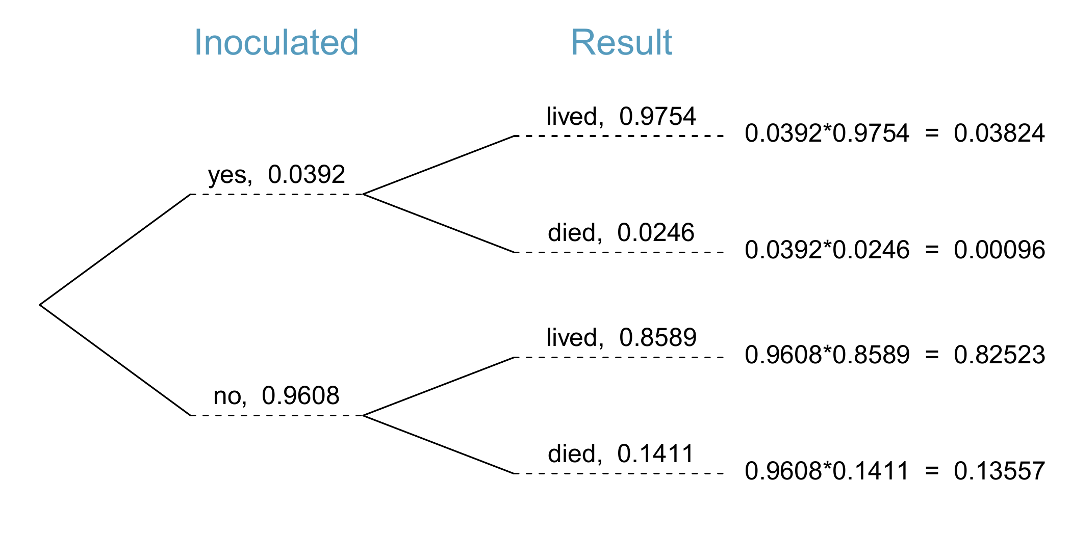
Figure 7.9: A tree diagram of the smallpox data set.

Tree diagrams are annotated with marginal and conditional probabilities, as shown in Figure 7.9. This tree diagram splits the smallpox data by $\texttt{inoculation}$ into the $\texttt{yes}$ and $\texttt{no}$ groups with respective marginal probabilities 0.0392 and 0.9608. The secondary branches are conditioned on the first, so we assign conditional probabilities to these branches. For example, the top branch in Figure 7.9 is the probability that $\texttt{result}$ = $\texttt{lived}$ conditioned on the information that $\texttt{inoculated}$ = $\texttt{yes}$. We may (and usually do) construct joint probabilities at the end of each branch in our tree by multiplying the numbers we come across as we move from left to right. These joint probabilities are computed using the General Multiplication Rule: \[ \begin{aligned} & P(\texttt{inoculated} = \texttt{yes}\text{ and }\texttt{result} = \texttt{lived}) \\ & = P(\texttt{inoculated} = \texttt{yes})\times P(\texttt{result} = \texttt{lived}|\texttt{inoculated} = \texttt{yes}) \\ & = 0.0392\times 0.9754=0.0382 \end{aligned} \]

Example 7.6 Consider the midterm and final exam for a statistics class. Suppose 13% of students earned an $\texttt{A}$ on the midterm. Of those students who earned an $\texttt{A}$ on the midterm, 47% received an $\texttt{A}$ on the final exam, and 11% of the students who earned lower than an $\texttt{A}$ on the midterm received an $\texttt{A}$ on the final. You randomly pick up a final exam and notice the student received an $\texttt{A}$. What is the probability that this student earned an $\texttt{A}$ on the midterm?

The end-goal is to find $P(\texttt{midterm} = \texttt{A} | \texttt{final} = \texttt{A})$. To calculate this conditional probability, we need the following probabilities: \[ P(\texttt{midterm} = \texttt{A} \text{ and } \texttt{final} = \texttt{A}) \text{ and } P(\texttt{final} = \texttt{A}) \] However, this information is not provided, and it is not obvious how to calculate these probabilities. Since we aren’t sure how to proceed, it is useful to organize the information into a tree diagram, as shown in Figure 7.10. When constructing a tree diagram, variables provided with marginal probabilities are often used to create the tree’s primary branches; in this case, the marginal probabilities are provided for midterm grades. The final grades, which correspond to the conditional probabilities provided, will be shown on the secondary branches.

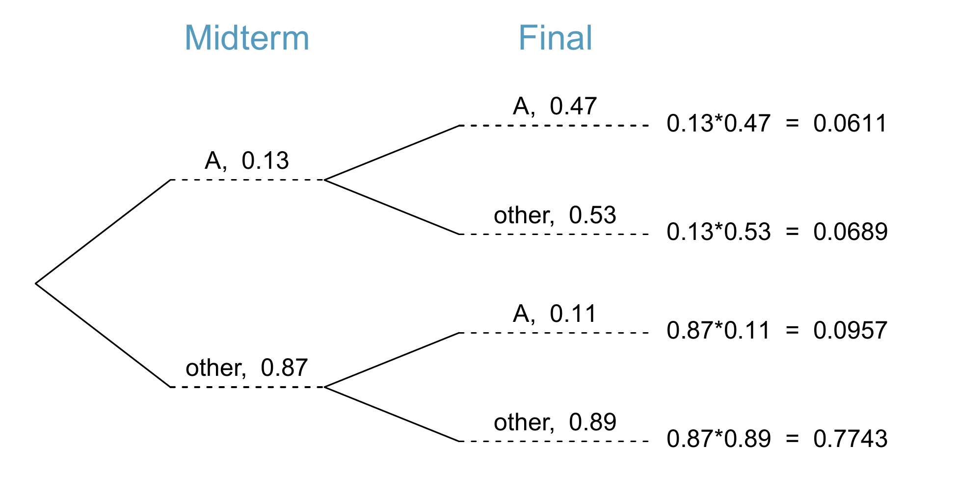
Figure 7.10: A tree diagram describing the midterm and final variables.

With the tree diagram constructed, we may compute the required probabilities: \[ \begin{aligned} &P(\texttt{midterm} = \texttt{A}\text{ and }\texttt{final} = \texttt{A}) = 0.0611 \\ P(\texttt{final} = \texttt{A}) &= P(\texttt{midterm} = \texttt{other}\text{ and } \texttt{final} = \texttt{A}) + P(\texttt{midterm} = \texttt{A}\text{ and } \texttt{final} = \texttt{A}) \\ &= 0.0957 + 0.0611 \\ &= 0.1568 \end{aligned} \] The marginal probability, $P(\texttt{final} = \texttt{A})$, was calculated by adding up all the joint probabilities on the right side of the tree that correspond to $\texttt{final} = \texttt{A}$. We may now finally take the ratio of the two probabilities: \[ \begin{aligned} &P(\texttt{midterm} = \texttt{A} | \texttt{final}= \texttt{A}) \\ =& \frac{P(\texttt{midterm} = \texttt{A}\text{ and }\texttt{final} = \texttt{A})}{P(\texttt{final} = \texttt{A})} \\ =& \frac{0.0611}{0.1568} = 0.3897 \end{aligned} \] The probability the student also earned an A on the midterm is about 0.39.

Guided Practice7.34 After an introductory statistics course, 78% of students can successfully construct tree diagrams. Of those who can construct tree diagrams, 97% passed, while only 57% of those students who could not construct tree diagrams passed.

Organize this information into a tree diagram.
What is the probability that a randomly selected student passed?
Compute the probability a student is able to construct a tree diagram if it is known that she passed.⁴⁵

7.2.7 Bayes’ Theorem

In many instances, we are given a conditional probability of the form \[ P(\text{statement about variable 1 } | \text{ statement about variable 2}) \] but we would really like to know the inverted conditional probability: \[ P(\text{statement about variable 2 } | \text{ statement about variable 1}) \] Tree diagrams can be used to find the second conditional probability when given the first. However, sometimes it is not possible to draw the scenario in a tree diagram. In these cases, we can apply a very useful and general formula: Bayes’ Theorem.

We first take a critical look at an example of inverting conditional probabilities where we still apply a tree diagram.

Example 7.7 In Canada, about 0.35% of women over 40 will develop breast cancer in any given year. A common screening test for cancer is the mammogram, but this test is not perfect. In about 11% of patients with breast cancer, the test gives a false negative: it indicates a woman does not have breast cancer when she does have breast cancer. Similarly, the test gives a false positive in 7% of patients who do not have breast cancer: it indicates these patients have breast cancer when they actually do not.⁴⁶

If we tested a random woman over 40 for breast cancer using a mammogram and the test came back positive – that is, the test suggested the patient has cancer – what is the probability that the patient actually has breast cancer?

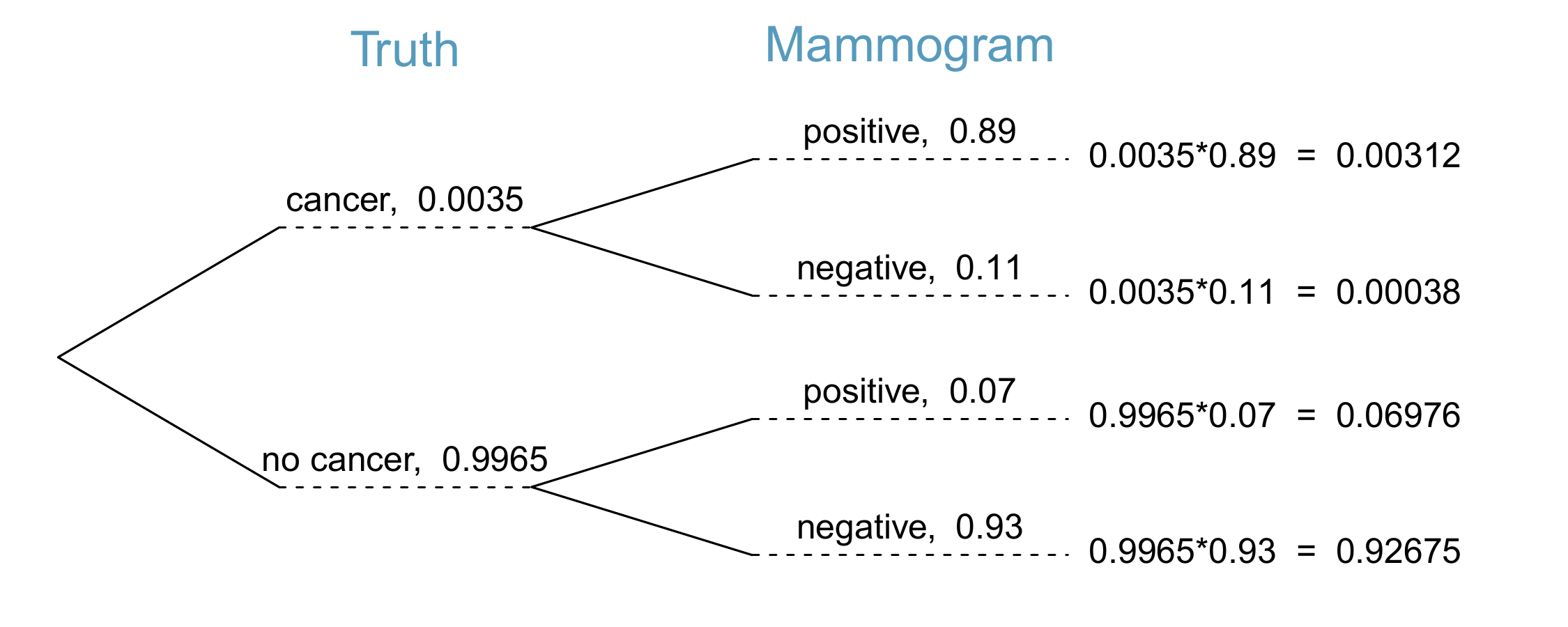
Figure 7.11: Tree diagram for Example 7.7, computing the probability a random patient who tests positive on a mammogram actually has breast cancer.

Notice that we are given sufficient information to quickly compute the probability of testing positive if a woman has breast cancer ($1.00-0.11=0.89$). However, we seek the inverted probability of cancer given a positive test result. (Watch out for the non-intuitive medical language: a positive test result suggests the possible presence of cancer in a mammogram screening.) This inverted probability may be broken into two pieces: \[ P(\text{has BC } | \text{ mammogram}^+) = \frac{P(\text{has BC and mammogram}^+)}{P(\text{mammogram}^+)} \]

where “has BC” is an abbreviation for the patient actually having breast cancer and “mammogram$^+$” means the mammogram screening was positive. A tree diagram is useful for identifying each probability and is shown in Figure 7.11. The probability the patient has breast cancer and the mammogram is positive is

\[ \begin{aligned} P(\text{has BC and mammogram}^+) &= P(\text{mammogram}^+ | \text{ has BC})P(\text{has BC}) \\ &= 0.89\times 0.0035 = 0.00312 \end{aligned} \] The probability of a positive test result is the sum of the two corresponding scenarios: \[ \begin{aligned} P(\text{mammogram}^+) &= P(\text{mammogram}^+\text{ and has BC}) + P(\text{mammogram}^+ \text{ and no BC}) \\ &= P(\text{has BC})P(\text{mammogram}^+ | \text{ has BC}) \\ &\qquad\qquad + P(\text{no BC})P(\text{mammogram}^+ | \text{ no BC}) \\ &= 0.0035\times 0.89 + 0.9965\times 0.07 = 0.07288 \end{aligned} \] Then if the mammogram screening is positive for a patient, the probability the patient has breast cancer is \[ \begin{aligned} P(\text{has BC } | \text{ mammogram}^+) &= \frac{P(\text{has BC and mammogram}^+)}{P(\text{mammogram}^+)}\\ &= \frac{0.00312}{0.07288} \approx 0.0428 \end{aligned} \] That is, even if a patient has a positive mammogram screening, there is still only a 4% chance that she has breast cancer.

Example 7.7 highlights why doctors often run more tests regardless of a first positive test result. When a medical condition is rare, a single positive test isn’t generally definitive.

Consider again the last equation of Example 7.7. Using the tree diagram, we can see that the numerator (the top of the fraction) is equal to the following product: \[ P(\text{has BC and mammogram}^+) = P(\text{mammogram}^+| \text{ has BC})P(\text{has BC}) \] The denominator – the probability the screening was positive – is equal to the sum of probabilities for each positive screening scenario: \[ P(\text{mammogram}^+) = P(\text{mammogram}^+\text{ and no BC}) + P(\text{mammogram}^+\text{ and has BC}) \] In the example, each of the probabilities on the right side was broken down into a product of a conditional probability and marginal probability using the tree diagram. \[ \begin{aligned} P(\text{mammogram}^+) &= P(\text{mammogram}^+ \text{ and no BC}) + P(\text{mammogram}^+\text{ and has BC}) \\ &= P(\text{mammogram}^+ | \text{ no BC})P(\text{no BC}) \\ &\qquad\qquad + P(\text{mammogram}^+ | \text{ has BC})P(\text{has BC}) \end{aligned} \] We can see an application of Bayes’ Theorem by substituting the resulting probability expressions into the numerator and denominator of the original conditional probability. \[ \begin{aligned} & P(\text{has BC } | \text{ mammogram}^+) \\ & \qquad= \frac{P(\text{mammogram}^+ | \text{ has BC})P(\text{has BC})} {P(\text{mammogram}^+ | \text{ no BC})P(\text{no BC}) + P(\text{mammogram}^+ | \text{ has BC})P(\text{has BC})} \end{aligned} \]

Definition 7.12 (Bayes’ Theorem: inverting probabilities) Consider the following conditional probability for variable 1 and variable \[ P(\text{outcome }A_1\text{ of variable 1 } | \text{ outcome }B\text{ of variable 2}) \] Bayes’ Theorem states that this conditional probability can be identified as the following fraction: \[ \frac{P(B | A_1) P(A_1)} {P(B | A_1) P(A_1) + P(B | A_2) P(A_2) + \cdots + P(B | A_k) P(A_k)} \tag{7.12} \] where $A_2$, $A_3$, …, and $A_k$ represent all other possible outcomes of the first variable.

Bayes’ Theorem is just a generalization of what we have done using tree diagrams. The numerator identifies the probability of getting both $A_1$ and $B$. The denominator is the marginal probability of getting $B$. This bottom component of the fraction appears long and complicated since we have to add up probabilities from all of the different ways to get $B$. We always completed this step when using tree diagrams. However, we usually did it in a separate step so it didn’t seem as complex.

To apply Bayes’ Theorem correctly, there are two preparatory steps:

First identify the marginal probabilities of each possible outcome of the first variable: $P(A_1)$, $P(A_2)$, …, $P(A_k)$.
Then identify the probability of the outcome $B$, conditioned on each possible scenario for the first variable: $P(B | A_1)$, $P(B | A_2)$, …, $P(B | A_k)$.

Once each of these probabilities are identified, they can be applied directly within the formula.

Remark (Only use Bayes’ Theorem when tree diagrams are difficult). Drawing a tree diagram makes it easier to understand how two variables are connected. Use Bayes’ Theorem only when there are so many scenarios that drawing a tree diagram would be complex.

Guided Practice7.35 Jose visits campus every Thursday evening. However, some days the parking garage is full, often due to college events. There are academic events on 35% of evenings, sporting events on 20% of evenings, and no events on 45% of evenings. When there is an academic event, the garage fills up about 25% of the time, and it fills up 70% of evenings with sporting events. On evenings when there are no events, it only fills up about 5% of the time. If Jose comes to campus and finds the garage full, what is the probability that there is a sporting event? Use a tree diagram to solve this problem.⁴⁷

Example 7.8 Here we solve the same problem presented in Guided Practice 7.35, except this time we use Bayes’ Theorem.

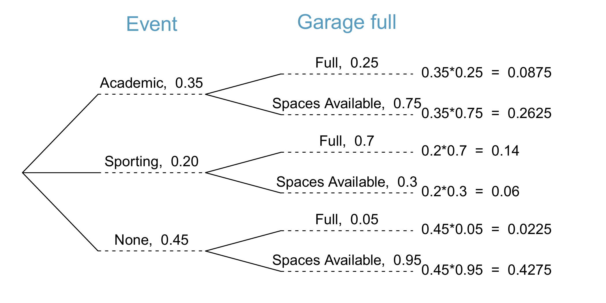
The outcome of interest is whether there is a sporting event (call this $A_1$), and the condition is that the lot is full ($B$). Let $A_2$ represent an academic event and $A_3$ represent there being no event on campus. Then the given probabilities can be written as \[ \begin{aligned} &P(A_1) = 0.2 &&P(A_2) = 0.35 &&P(A_3) = 0.45 \\ &P(B | A_1) = 0.7 &&P(B | A_2) = 0.25 &&P(B | A_3) = 0.05 \end{aligned} \] Bayes’ Theorem can be used to compute the probability of a sporting event ($A_1$) under the condition that the parking lot is full ($B$): \[ \begin{aligned} P(A_1 | B) &= \frac{P(B | A_1) P(A_1)}{P(B | A_1) P(A_1) + P(B | A_2) P(A_2) + P(B | A_3) P(A_3)} \\ &= \frac{(0.7)(0.2)}{(0.7)(0.2) + (0.25)(0.35) + (0.05)(0.45)} \\ &= 0.56 \end{aligned} \] Based on the information that the garage is full, there is a 56% probability that a sporting event is being held on campus that evening.

Guided Practice7.36 Use the information in the previous exercise and example to verify the probability that there is an academic event conditioned on the parking lot being full is 0.35.⁴⁸

Guided Practice7.37 In Guided Practice 7.35 and 7.36, you found that if the parking lot is full, the probability there is a sporting event is 0.56 and the probability there is an academic event is 0.35. Using this information, compute $P($no event $|$ the lot is full$)$.⁴⁹

The last several exercises offered a way to update our belief about whether there is a sporting event, academic event, or no event going on at the school based on the information that the parking lot was full. This strategy of updating beliefs using Bayes’ Theorem is actually the foundation of an entire section of statistics called Bayesian statistics. While Bayesian statistics is very important and useful, we will not have time to cover much more of it in this book.

If the die is fair, then the chance of a $1$ is as good as the chance of any other number. Since there are six outcomes, the chance must be 1-in-6 or, equivalently, $1/6$.↩︎
$1$ and $2$ constitute two of the six equally likely possible outcomes, so the chance of getting one of these two outcomes must be $2/6 = 1/3$.↩︎
100%. The outcome must be one of these numbers.↩︎
Since the chance of rolling a $2$ is $1/6$ or $16.\bar{6}\%$, the chance of not rolling a $2$ must be $100\% - 16.\bar{6}\%=83.\bar{3}\%$ or $5/6$. Alternatively, we could have noticed that not rolling a $2$ is the same as getting a $1$, $3$, $4$, $5$, or $6$, which makes up five of the six equally likely outcomes and has probability $5/6$.↩︎
If $16.\bar{6}$% of the time the first die is a $1$ and $1/6^{th}$ of those times the second die is also a $1$, then the chance that both dice are $1$ is $(1/6)\times (1/6)$ or $1/36$.↩︎
Here are four examples: (i) Whether someone gets sick in the next month or not is an apparently random process with outcomes sick and not. (ii) We can generate a random process by randomly picking a person and measuring that person’s height. The outcome of this process will be a positive number. (iii) Whether the stock market goes up or down next week is a seemingly random process with possible outcomes up, down, and no change. Alternatively, we could have used the percent change in the stock market as a numerical outcome. (iv) Whether your housemate cleans her dishes tonight probably seems like a random process with possible outcomes cleans dishes and leaves dishes.↩︎
(a) the random process is a die roll, and at most one of these outcomes can come up. This means they are disjoint outcomes. (b) $P(1\textrm{ or }4\textrm{ or }5) = P(1)+P(4)+P(5)$ $= \frac{1}{6} + \frac{1}{6} + \frac{1}{6}$ $= \frac{3}{6} = \frac{1}{2}$↩︎
(a) Yes. Each email is categorized in only one level of number. (b) Small: $\frac{2827}{3921} = 0.721$. Big: $\frac{545}{3921} = 0.139$. (c) $P(small\textrm{ or } big) = P(small) + P(big) = 0.721 + 0.139 = 0.860$.↩︎
(a) Outcomes $2$ and $3$. (b) Yes, events $B$ and $D$ are disjoint because they share no outcomes. (c) The events $A$ and $D$ share an outcome in common, $2$, and so are not disjoint.↩︎
Since $B$ and $D$ are disjoint events, use the Addition Rule: $P(B \text{ or } D) = P(B) + P(D) = \frac{1}{3} + \frac{1}{3} = \frac{2}{3}$↩︎
The 52 cards are split into four suits: $\clubsuit$ (club), $\color{red}\diamondsuit$ (diamond), $\color{red}\heartsuit$ (heart), $\spadesuit$ (spade). Each suit has its 13 cards labeled: $2,3,\ldots,10,J\text{ (jack)},Q\text{ (queen)},K\text{ (king) and }$A$\text{( ace)}$. Thus, each card is a unique combination of a suit and a label, e.g. $\color{red}{4\heartsuit}$ and $J\clubsuit$. The 12 cards represented by the jacks, queens, and kings are called face cards. The cards that are $\color{red}{\diamondsuit}$ or $\color{red}\heartsuit$ are typically coloured $\color{red}{red}$ while the other two suits are typically colored black.↩︎
(a) There are 52 cards and 13 diamonds. If the cards are thoroughly shuffled, each card has an equal chance of being drawn, so the probability that a randomly selected card is a diamond is $P({\color{red}\diamondsuit}) = \frac{13}{52} = 0.250$. (b) Likewise, there are 12 face cards, so $P($face card$) = \frac{12}{52} = \frac{3}{13} = 0.231$.↩︎
The Venn diagram shows face cards split up into “face card but not $\color{red}\diamondsuit$” and “face card and $\color{red}\diamondsuit$.” Since these correspond to disjoint events, $P(\text{face card})$ is found by adding the two corresponding probabilities: $\frac{3}{52} + \frac{9}{52} = \frac{12}{52} = \frac{3}{13}$.↩︎
(a) If $A$ and $B$ are disjoint, $A$ and $B$ can never occur simultaneously. (b) If $A$ and $B$ are disjoint, then the last term of Equation (7.3) is 0 (see part (a)) and we are left with the Addition Rule for disjoint events.↩︎
(a) The solution is represented by the intersection of the two circles: 0.043. (b) This is the sum of the three disjoint probabilities shown in the circles: $0.678 + 0.043 + 0.051 = 0.772$.↩︎
The probabilities of (c) do not sum to 1. The second probability in (b) is negative. This leaves (a), which sure enough satisfies the requirements of a distribution. One of the three was said to be the actual distribution of Australian household incomes, so it must be (a).↩︎
http://www.abs.gov.au/AUSSTATS/abs@.nsf/DetailsPage/6523.02013-14?OpenDocument ↩︎
(a) The outcomes are disjoint and each has probability $1/6$, so the total probability is $4/6=2/3$. (b) We can also see that $P(D)=\frac{1}{6} + \frac{1}{6} = 1/3$. Since $D$ and $D^c$ are disjoint, $P(D) + P(D^c) = 1$.↩︎
Brief solutions: (a) $A^c=\{3, 4, 5, 6\}$ and $B^c=\{1,2,3,5\}$. (b) Noting that each outcome is disjoint, add the individual outcome probabilities to get $P(A^c)=2/3$ and $P(B^c)=2/3$. (c) $A$ and $A^c$ are disjoint, and the same is true of $B$ and $B^c$. Therefore, $P(A) + P(A^c) = 1$ and $P(B) + P(B^c) = 1$.↩︎
(a) The complement of $A$: when the total is equal to $12$. (b) $P(A^c) = 1/36$. (c) Use the probability of the complement from part (b), $P(A^c) = 1/36$, and Equation (7.6): $P(\text{less than }12) = 1 - P(12) = 1 - 1/36 = 35/36$.↩︎
(a) First find $P(6)=5/36$, then use the complement: $P(\text{not }6) = 1 - P(6) = 31/36$. (b) First find the complement, which requires much less effort: $P(2 \text{ or }3)=1/36+2/36=1/12$. Then calculate $P(B) = 1-P(B^c) = 1-1/12 = 11/12$. (c) As before, finding the complement is the clever way to determine $P(D)$. First find $P(D^c) = P(11\text{ or }12)=2/36 + 1/36=1/12$. Then calculate $P(D) = 1 - P(D^c) = 11/12$.↩︎
A simulated data set based on real population summaries at www.nces.ed.gov/pubs2001/2001126.pdf .↩︎
Each of the four outcome combination are disjoint, all probabilities are indeed non-negative, and the sum of the probabilities is $0.29 + 0.06 + 0.27 + 0.38 = 1.00$.↩︎
(a) $P(parents=not | teen=not)$. (b) Equation (7.11) for conditional probability indicates we should first find \[P(parents = not \text{ and }teen = not) = 0.38\] and \[P(teen = not) = 0.44\]. Then the ratio represents the conditional probability: $0.38 / 0.44 = 0.864$.↩︎
(a) This probability is $\frac{P(parents = degree, teen = not)}{P(teen = not)} = \frac{0.06}{0.44} = 0.136$. (b) The total equals 1. (c) Under the condition the teenager didn’t attend college, the parents must either have a college degree or not. The complement still works for conditional probabilities, provided the probabilities are conditioned on the same information.↩︎
No. While there is an association, the data are observational. Two potential confounding variables include income and region. Can you think of others?↩︎
Fenner F. 1988. Smallpox and Its Eradication (History of International Public Health, No. 6). Geneva: World Health Organization. ISBN 92-4-156110-6.↩︎
$P(result = died | inoculated = no) = \frac{P(result = died\text{ and }inoculated = no)}{P(inoculated = no)} = \frac{0.1356}{0.9608} = 0.1411$.↩︎
$P(result = died | inoculated = yes) = \frac{P(result = died\text{ and }inoculated = yes)}{P(inoculated = yes)} = \frac{0.0010}{0.0392} = 0.0255$. The death rate for individuals who were inoculated is only about 1 in 40 while the death rate is about 1 in 7 for those who were not inoculated.↩︎
Brief answers: (a) Observational. (b) No, we cannot infer causation from this observational study. (c) Accessibility to the latest and best medical care. There are other valid answers for part (c).↩︎
The answer is 0.0382, which can be verified using Table 7.8.↩︎
There were only two possible outcomes: $lived$ or $died$. This means that 100% - 97.45% = 2.55% of the people who were inoculated died.↩︎
The samples are large relative to the difference in death rates for the “inoculated” and “not inoculated” groups, so it seems there is an association between $inoculated$ and $outcome$. However, as noted in the solution to Guided Practice 7.28, this is an observational study and we cannot be sure if there is a causal connection. (Further research has shown that inoculation is effective at reducing death rates.)↩︎
Brief solutions: (a) $1/6$. (b) $1/36$. (c) $\frac{P(Y = 1 \text{ and }X=1)}{P(X=1)} = \frac{1/36}{1/6} = 1/6$. (d) The probability is the same as in part (c): $P(Y=1)=1/6$. The probability that $Y=1$ was unchanged by knowledge about $X$, which makes sense as $X$ and $Y$ are independent.↩︎
He has forgotten that the next roulette spin is independent of the previous spins. Casinos do employ this practice; they post the last several outcomes of many betting games to trick unsuspecting gamblers into believing the odds are in their favor. This is called the gambler’s fallacy↩︎
(a) 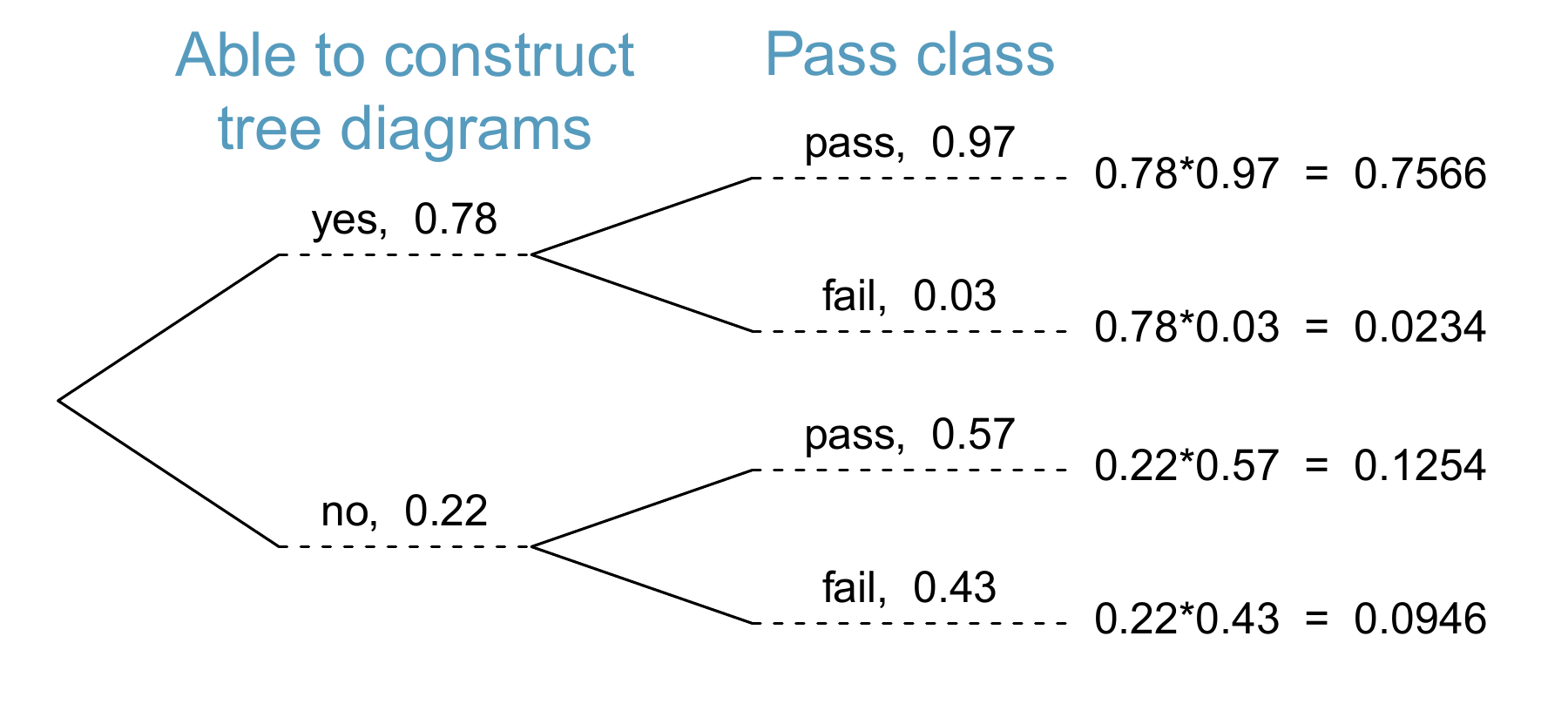(b) Identify which two joint probabilities represent students who passed, and add them: $P(\texttt{passed}) = 0.7566+0.1254= 0.8820$. (c) $P(\text{construct tree diagram }| \texttt{passed}) = \frac{0.7566}{0.8820} = 0.8578$.↩︎
The probabilities reported here were obtained using studies reported at www.breastcancer.org and www.ncbi.nlm.nih.gov/pmc/articles/PMC1173421 .↩︎
The tree diagram, with three primary branches, is shown to the right. Next, we identify two probabilities from the tree diagram. (1) The probability that there is a sporting event and the garage is full: 0.14. (2) The probability the garage is full: $0.0875 + 0.14 + 0.0225 = 0.25$. Then the solution is the ratio of these probabilities: $\frac{0.14}{0.25} = 0.56$. If the garage is full, there is a 56% probability that there is a sporting event. ↩︎
Short answer: \[ \begin{aligned} P(A_2 | B) &= \frac{P(B | A_2) P(A_2)}{P(B | A_1) P(A_1) + P(B | A_2) P(A_2) + P(B | A_3) P(A_3)} \\ &= \frac{(0.25)(0.35)}{(0.7)(0.2) + (0.25)(0.35) + (0.05)(0.45)} \\ &= 0.35 \end{aligned} \]↩︎
Each probability is conditioned on the same information that the garage is full, so the complement may be used: $1.00 - 0.56 - 0.35 = 0.09$.↩︎

Action	\(\rightarrow\)	Outcome
Roll a die	\(\rightarrow\)	\(1,2,3,4,5\) or \(6\)
Flip a coin	\(\rightarrow\)	\(H\) or \(T\)

\(2\clubsuit\)	\(3\clubsuit\)	\(4\clubsuit\)	\(5\clubsuit\)	\(6\clubsuit\)	\(7\clubsuit\)	\(8\clubsuit\)	\(9\clubsuit\)	\(10\clubsuit\)	\(J\clubsuit\)	\(Q\clubsuit\)	\(K\clubsuit\)	\(A\clubsuit\)
\(\color{red}{2\diamondsuit}\)	\(\color{red}{3\diamondsuit}\)	\(\color{red}{4\diamondsuit}\)	\(\color{red}{5\diamondsuit}\)	\(\color{red}{6\diamondsuit}\)	\(\color{red}{7\diamondsuit}\)	\(\color{red}{8\diamondsuit}\)	\(\color{red}{9\diamondsuit}\)	\(\color{red}{10\diamondsuit}\)	\(\color{red}{J\diamondsuit}\)	\(\color{red}{Q\diamondsuit}\)	\(\color{red}{K\diamondsuit}\)	\(\color{red}{A\diamondsuit}\)
\(\color{red}{2\heartsuit}\)	\(\color{red}{3\heartsuit}\)	\(\color{red}{4\heartsuit}\)	\(\color{red}{5\heartsuit}\)	\(\color{red}{6\heartsuit}\)	\(\color{red}{7\heartsuit}\)	\(\color{red}{8\heartsuit}\)	\(\color{red}{9\heartsuit}\)	\(\color{red}{10\heartsuit}\)	\(\color{red}{J\heartsuit}\)	\(\color{red}{Q\heartsuit}\)	\(\color{red}{K\heartsuit}\)	\(\color{red}{A\heartsuit}\)
\(2\spadesuit\)	\(3\spadesuit\)	\(4\spadesuit\)	\(5\spadesuit\)	\(6\spadesuit\)	\(7\spadesuit\)	\(8\spadesuit\)	\(9\spadesuit\)	\(10\spadesuit\)	\(J\spadesuit\)	\(Q\spadesuit\)	\(K\spadesuit\)	\(A\spadesuit\)