Chapter 2 Introduction to Data

Scientists seek to answer questions using rigorous methods and careful observations. These observations – collected from the likes of field notes, surveys, and experiments – form the backbone of a statistical investigation and are called data. Statistics is the study of how best to collect, analyse, and draw conclusions from data. It is helpful to put statistics in the context of a general process of investigation:

Identify a question or problem.
Collect relevant data on the topic.
Analyse the data.
Form a conclusion.

Statistics as a subject focuses on making stages 2-4 objective, rigorous, and efficient. That is, statistics has three primary components: How best can we collect data? How should it be analysed? And what can we infer from the analysis?

The topics scientists investigate are as diverse as the questions they ask. However, many of these investigations can be addressed with a small number of data collection techniques, analytic tools, and fundamental concepts in statistical inference. This chapter provides a glimpse into these and other themes we will encounter throughout the rest of the book. We introduce the basic principles of each branch and learn some tools along the way. We will encounter applications from other fields, some of which are not typically associated with science but nonetheless can benefit from statistical study.

2.1 Case Study: Using stents to prevent strokes

This section introduces a classic challenge in statistics: evaluating the efficacy of a medical treatment. Terms in this section, and indeed much of this chapter, will all be revisited later in the text. The plan for now is simply to get a sense of the role statistics can play in practice.

In this section we will consider an experiment that studies effectiveness of stents in treating patients at risk of stroke.¹

Stents are devices put inside blood vessels that assist in patient recovery after cardiac events and reduce the risk of an additional heart attack or death. Many doctors have hoped that there would be similar benefits for patients at risk of stroke. We start by writing the principal question the researchers hope to answer:

Does the use of stents reduce the risk of stroke?

The researchers who asked this question collected data on 451 at-risk patients. Each volunteer patient was randomly assigned to one of two groups:

Treatment group Patients in the treatment group received a stent and medical management. The medical management included medications, management of risk factors, and help in lifestyle modification.
Control group Patients in the control group received the same medical management as the treatment group, but they did not receive stents.

Researchers randomly assigned 224 patients to the treatment group and 227 to the control group. In this study, the control group provides a reference point against which we can measure the medical impact of stents in the treatment group.

Researchers studied the effect of stents at two time points: 30 days after enrolment and 365 days after enrolment. The results of 5 patients are summarized in Table 2.1. Patient outcomes are recorded as “stroke” or “no event,” representing whether or not the patient had a stroke at the end of a time period.

Table 2.1: Stent study data overview
Patient	Group	0-30 days	0-365 days
1	treatment	no event	no event
2	treatment	stroke	stroke
3	treatment	stroke	stroke
$\vdots$	$\vdots$	$\vdots$	$\vdots$
450	control	no event	no event
451	control	no event	no event

Considering data from each patient individually would be a long, cumbersome path towards answering the original research question. Instead, performing a statistical data analysis allows us to consider all of the data at once. Table 2.2 summarizes the raw data in a more helpful way. In this table, we can quickly see what happened over the entire study. For instance, to identify the number of patients in the treatment group who had a stroke within 30 days, we look on the left-side of the table at the intersection of the treatment and stroke: 33.

Table 2.2: Descriptive statistics for the stent study
	0-30	days	0-365	days
	stroke	no event	stroke	no event
treatment	33	191	45	179
control	13	214	28	199
Total	46	405	73	378

Guided Practice2.1 Of the 224 patients in the treatment group, 45 had a stroke by the end of the first year. Using these two numbers, compute the proportion of patients in the treatment group who had a stroke by the end of their first year. (Please note: answers to all Guided Practice exercises are provided using footnotes, so follow this link $\nearrow$²)

We can compute summary statistics from the table. A summary statistic is a single number summarizing a large amount of data.³. For instance, the primary results of the study after 1~year could be described by two summary statistics: the proportion of people who had a stroke in the treatment and control groups.

Proportion who had a stroke in the treatment (stent) group: \[45/224 = 0.20 = 20\%\]
Proportion who had a stroke in the control group: \[28/227 = 0.12 = 12\%\]

These two summary statistics are useful in looking for differences in the groups, and we are in for a surprise: an additional 8% of patients in the treatment group had a stroke! This is important for two reasons. First, it is contrary to what doctors expected, which was that stents would reduce the rate of strokes. Second, it leads to a statistical question: do the data show a “real” difference between the groups?

This second question is subtle. Suppose you flip a coin 100 times. While the chance a coin lands heads in any given coin flip is 50%, we probably won’t observe exactly 50 heads. This type of fluctuation is part of almost any type of data generating process. It is possible that the 8% difference in the stent study is due to this natural variation. However, the larger the difference we observe (for a particular sample size), the less believable it is that the difference is due to chance. So what we are really asking is the following: is the difference so large that we should reject the notion that it was due to chance?

While we don’t yet have our statistical tools to fully address this question on our own, we can comprehend the conclusions of the published analysis: there was compelling evidence of harm by stents in this study of stroke patients.

Be careful: do not generalize the results of this study to all patients and all stents. This study looked at patients with very specific characteristics who volunteered to be a part of this study and who may not be representative of all stroke patients. In addition, there are many types of stents and this study only considered the self-expanding Wingspan stent (Boston Scientific). However, this study does leave us with an important lesson: we should keep our eyes open for surprises.

2.2 Data Basics

Effective presentation and description of data is a first step in most analyses. This section introduces one structure for organizing data as well as some terminology that will be used throughout this book.

Observations, variables, and data matrices

Table 2.3 displays rows 1, 2, 3, and 50 of a data set concerning 50 emails received during early 2012. These observations will be referred to as the email50 data set, and they are a random sample from a larger data set.

Each row in the table represents a single email or case⁴. The columns represent characteristics, called variables, for each of the emails. For example, the first row represents email 1, which is a not spam, contains 21,705 characters, 551 line breaks, is written in HTML format, and contains only small numbers.

The columns represent characteristics, called variables, for each of the emails. For example, the first row represents email 1, which is a not spam, contains 21,705 characters, 551 line breaks, is written in HTML format, and contains only small numbers.

In practice, it is especially important to ask clarifying questions to ensure important aspects of the data are understood. For instance, it is always important to be sure we know what each variable means and the units of measurement. Descriptions of all five email variables are given in Table 2.4.

Table 2.3: Four rows from the `email50` data matrix.
	spam	num char	line breaks	format	number
1	no	21,705	551	html	small
2	no	7,011	183	html	big
3	yes	631	28	text	none
$\vdots$	$\vdots$	$\vdots$	$\vdots$	$\vdots$	$\vdots$
50	no	15,829	242	html	small

Table 2.4: Variables and their descriptions for the `email50` data set.
variable	description
spam	Specifies whether the message was spam
num_char	The number of characters in the email
line_breaks	The number of line breaks in the email (not including text wrapping)
format	Indicates if the email contained special formatting, such as bolding, tables, or links, which would indicate the message is in HTML format
number	Indicates whether the email contained no number, a small number (under 1 million), or a large number

The data in Table 2.3 represent a data matrix, which is a common way to organize data. Each row of a data matrix corresponds to a unique case, and each column corresponds to a variable. A data matrix for the stroke study introduced in Section 2.1 is shown in Table 2.1, where the cases were patients and there were three variables recorded for each patient.

Data matrices are a convenient way to record and store data. If another individual or case is added to the data set, an additional row can be easily added. Similarly, another column can be added for a new variable.

Guided Practice2.2 We consider a publicly available data set that summarizes information about the 2,240 areas (known as “Statistical Area 2”) in Australia, and we call this the Census2016_wide_by_SA2_year data set⁵. This data set includes information about each SA2: its name, the state where it resides, its population in 2006,2011 and 2016 and many other characteristics. How might these data be organized in a data matrix? Reminder: look in the footnotes for answers to in-text exercises.⁶

Table 2.5: First 11 rows of 2016 Census area data set for selected variables
sa2_code	sa2_name	persons	prop_units	mortgage	income
501011001	Augusta	5431	Mid	21600	61672
501011002	Busselton	26334	Low	21600	62296
501011003	Busselton Region	10280	Low	24000	83876
501011004	Margaret River	8830	Low	20796	70408
501021005	Australind - Leschenault	17592	Mid	22644	87620
501021007	Capel	5195	Mid	20796	71864
501021008	College Grove - Carey Park	6746	Low	18204	55796
501021009	Collie	8798	Low	18204	60164
501021010	Dardanup	3142	Low	24000	85020
501021011	Davenport	9	Low	0	136500
501021012	Eaton - Pelican Point	11756	Low	21840	80652

2.2.1 Types of variables

Examine the $\texttt{mortgage}$ , $\texttt{persons}$ , $\texttt{sa2}\_\texttt{name}$ , and $\texttt{year}$ variables in the Census2016_wide_by_SA2_year data set. Each of these variables is inherently different from the other three yet many of them share certain characteristics.

First consider $\texttt{mortgage}$ which is said to be a numerical variable since it can take a wide range of numerical values, and it is sensible to add, subtract, or take averages with those values. On the other hand, we would not classify a variable reporting telephone area codes as numerical since their average, sum, and difference have no clear meaning.

The $\texttt{persons}$ variable is also numerical, although it seems to be a little different than $\texttt{mortgage}$. This variable of the population count can only take whole non-negative numbers $(0,1,2,\ldots)$. For this reason, the population variable is said to be discrete since it can only take numerical values with jumps. On the other hand, the $\texttt{mortgage}$ variable is said to be continuous.

The variable $\texttt{sa2}\_\texttt{name}$ can take up to 2240 values as these are one level of the statistical areas into which Australia can be divided. Because the responses themselves are categories, $\texttt{sa2}\_\texttt{name}$ is called a categorical variable, and the possible values are called the variable’s levels.

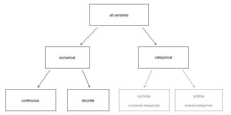
Figure 2.1: Breakdown of variables into their respective types.

Finally, consider the $\texttt{prop}\_\texttt{units}$ variable, which describes the proportion of dwellings in the area that are units or flats and takes values $\texttt{Low}$, $\texttt{Mid}$, or $\texttt{High}$ in area. This variable seems to be a hybrid: it is a categorical variable but the levels have a natural ordering. A variable with these properties is called an ordinal variable, while a regular categorical variable without this type of special ordering is called a nominal variable. To simplify analyses, any ordinal variables in this book will be treated as categorical variables.

Example 2.1 Data were collected about students in a statistics course. Three variables were recorded for each student: number of siblings, student height, and whether the student had previously taken a statistics course. Classify each of the variables as continuous numerical, discrete numerical, or categorical.

The number of siblings and student height represent numerical variables. Because the number of siblings is a count, it is discrete. Height varies continuously, so it is a continuous numerical variable. The last variable classifies students into two categories – those who have and those who have not taken a statistics course – which makes this variable categorical.

Guided Practice2.3 Consider the variables $\texttt{group}$ and $\texttt{outcome}$ (at 30 days) from the stent study in Section 2.1. Are these numerical or categorical variables?⁷

2.3 Relationships between variables

Many analyses are motivated by a researcher looking for a relationship between two or more variables. A social scientist may like to answer some of the following questions:

Are median rents related to proportion of dwellings that are units or flats?
If homeownership is lower than the national average in one area, will the percent of units or flats in that area likely be above or below the national average?
Which counties have a higher average income: those with more people born overseas or not?

To answer these questions, data must be collected, such as the Census2016_wide_by_SA2_year data set shown in Table 2.5. Examining summary statistics could provide insights for each of the three questions about areas. Additionally, graphs can be used to visually summarize data and are useful for answering such questions as well.

Definition 2.1 (Scatterplots) Scatterplots are one type of graph used to study the relationship between two numerical variables. Figure 2.2 compares the variables $\texttt{mortgage}$ and $\texttt{income}$. Each point on the plot represents a single area at the SA2 level. For instance, the highlighted dot corresponds to SA2 503011035 in the Census2016_wide_by_SA2_year data set: {"Nedlands - Dalkeith - Crawley"}, which had a median household income of $118,976 and median annual mortgage of $39,600. The scatterplot suggests a relationship between the two variables: SA2s with higher incomes tend to have higher mortgages.

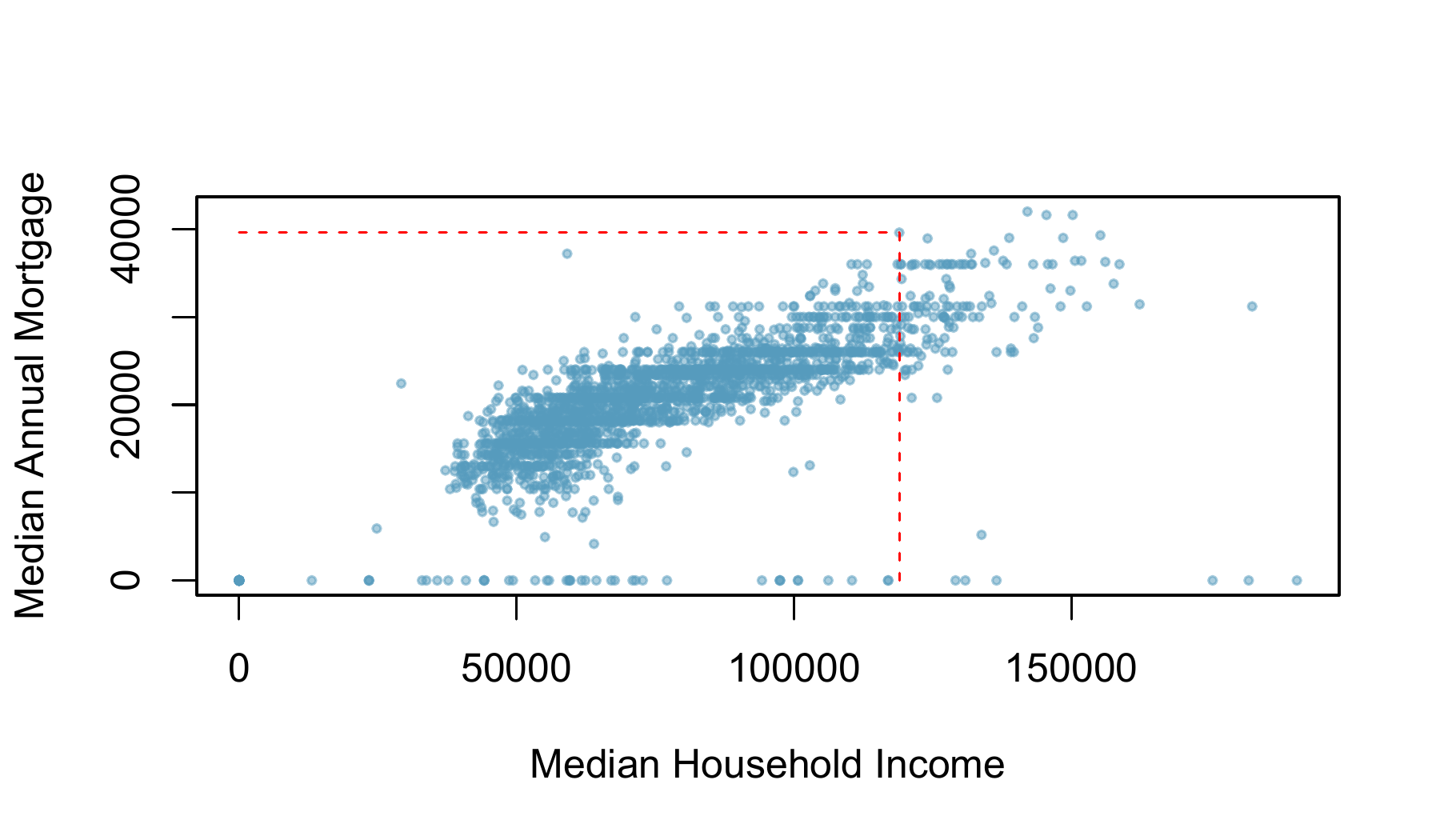
$A scatterplot showing $\texttt{mortgage}$ against $\texttt{income}$. The statistical area surrounding UWA, with median household income of $118,976 and median annual mortgage of $39,600, is highlighted$

Figure 2.2: A scatterplot showing $\texttt{mortgage}$ against $\texttt{income}$. The statistical area surrounding UWA, with median household income of $118,976 and median annual mortgage of $39,600, is highlighted

Guided Practice2.4 Examine the variables in the email50 data set, which are described in Table 2.4. Create two questions about the relationships between these variables that are of interest to you.⁸

If two variables are not associated, then they are said to be independent. That is, two variables are independent if there is no evident relationship between the two.

Definition 2.2 (Associated or independent, not both) A pair of variables are either related in some way (associated) or not (independent). No pair of variables is both associated and independent.}

2.4 Overview of Data Collection Principles

The first step in conducting research is to identify topics or questions that are to be investigated. A clearly laid out research question is helpful in identifying what subjects or cases should be studied and what variables are important. It is also important to consider how data are collected so that they are reliable and help achieve the research goals.

Populations and samples

Consider the following three research questions:

What is the average mercury content in swordfish in the Atlantic Ocean?
Over the last 5 years, what is the average time to complete a degree for UWA undergraduate students?
Does a new drug reduce the number of deaths in patients with severe heart disease?

Each research question refers to a target population. In the first question, the target population is all swordfish in the Atlantic ocean, and each fish represents a case. Often times, it is too expensive to collect data for every case in a population. Instead, a sample is taken. A sample represents a subset of the cases and is often a small fraction of the population. For instance, 60 swordfish (or some other number) in the population might be selected, and this sample data may be used to provide an estimate of the population average and answer the research question.

Guided Practice2.5 For the second and third questions above, identify the target population and what represents an individual case.⁹

2.5 Sampling from a population

We might try to estimate the time to graduation for UWA undergraduates in the last 5 years by collecting a sample of students. All graduates in the last 5 years represent the population, and graduates who are selected for review are collectively called the sample. In general, we always seek to randomly select a sample from a population. The most basic type of random selection is equivalent to how raffles are conducted. For example, in selecting graduates, we could write each graduate’s name on a raffle ticket and draw 100 tickets. The selected names would represent a random sample of 100 graduates.

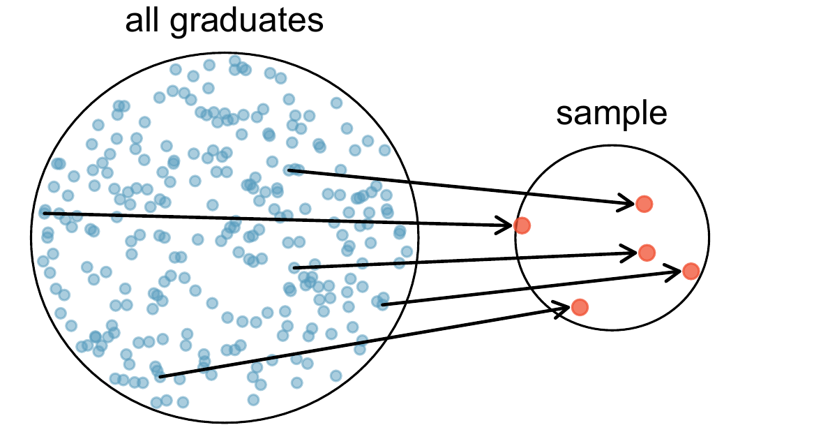
Figure 2.3: In this graphic, five graduates are randomly selected from the population to be included in the sample.

Why pick a sample randomly? Why not just pick a sample by hand? Consider the following scenario.

Example 2.2 Suppose we ask a student who happens to be majoring in nutrition to select several graduates for the study. What kind of students do you think she might collect? Do you think her sample would be representative of all graduates?

Perhaps she would pick a disproportionate number of graduates from health-related fields. Or perhaps her selection would be well-representative of the population. When selecting samples by hand, we run the risk of picking a sample, even if that bias is unintentional or difficult to discern.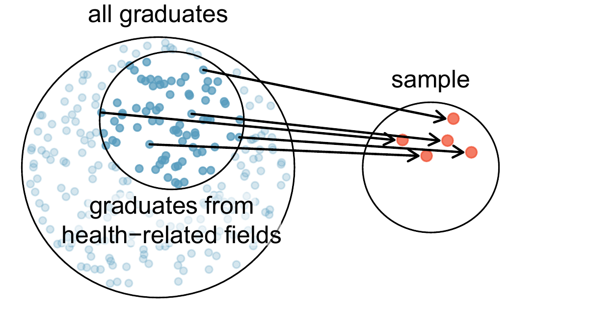

Instead of sampling from all graduates equally, a nutrition major might inadvertently pick graduates with health-related majors disproportionately often.

Figure 2.4: Instead of sampling from all graduates equally, a nutrition major might inadvertently pick graduates with health-related majors disproportionately often.

If someone was permitted to pick and choose exactly which graduates were included in the sample, it is entirely possible that the sample could be skewed to that person’s interests, which may be entirely unintentional. This introduces bias into a sample. Sampling randomly helps resolve this problem. The most basic random sample is called a simple random sample, and is equivalent to using a raffle to select cases. This means that each case in the population has an equal chance of being included and there is no implied connection between the cases in the sample.

Sometimes a simple random sample is difficult to implement and an alternative method is helpful. One such substitute is a systematic sample, where one case is sampled after letting a fixed number of others, say 10 other cases, pass by. Since this approach uses a mechanism that is not easily subject to personal biases, it often yields a reasonably representative sample. This book will focus on random samples since the use of systematic samples is less common and requires additional considerations of the context.

The act of taking a simple random sample helps minimize bias, however, bias can crop up in other ways. Even when people are picked at random, e.g. for surveys, caution must be exercised if the non-response is high. For instance, if only 30% of the people randomly sampled for a survey actually respond, then it is unclear whether the results are representative of the entire population. This non-response bias can skew results.

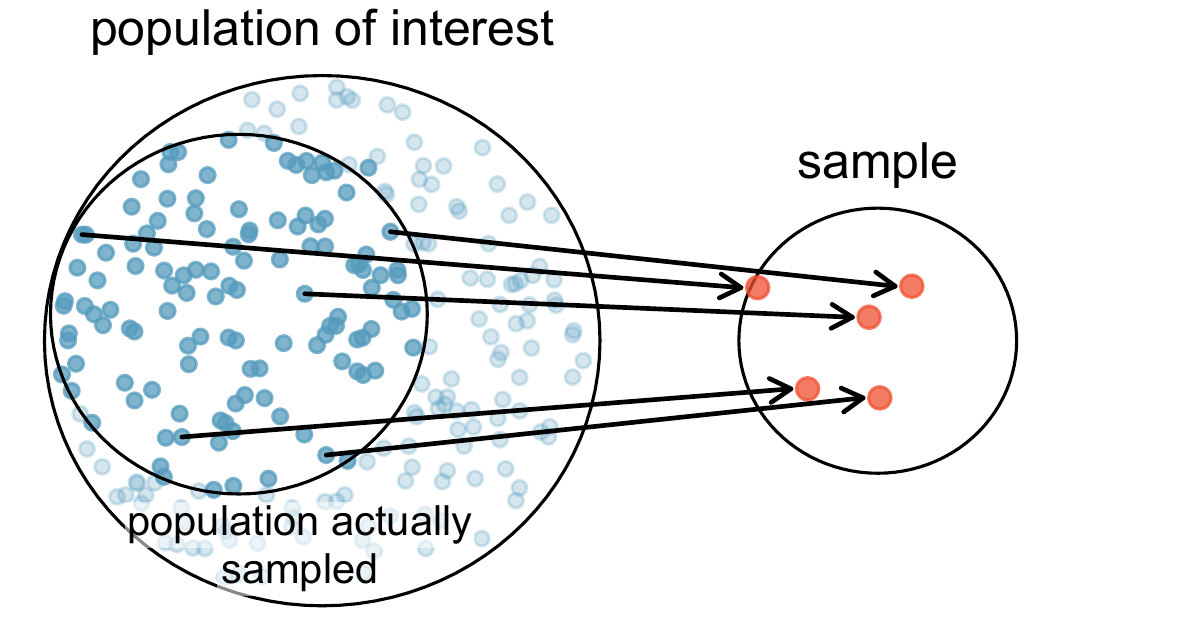
Due to the possibility of non-response, surveys studies may only reach a certain group within the population. It is difficult, and often times impossible, to completely fix this problem.

Figure 2.5: Due to the possibility of non-response, surveys studies may only reach a certain group within the population. It is difficult, and often times impossible, to completely fix this problem.

Introducing observational studies and experiments

There are two primary types of data collection: observational studies and experiments.

Researchers perform an observational study when they collect data in a way that does not directly interfere with how the data arise. For instance, researchers may collect information via surveys, review medical or company records, or follow a cohort of many similar individuals to study why certain diseases might develop. In each of these situations, researchers merely observe the data that arise. In general, observational studies can provide evidence of a naturally occurring association between variables. The methods used to establish causal connections in observational study data are complex, and continue to be debated.

When researchers want to investigate the possibility of a causal connection, they conduct an experiment. Usually there will be both an explanatory and a response variable. For instance, we may suspect administering a drug will reduce mortality in heart attack patients over the following year. To check if there really is a causal connection between the explanatory variable and the response, researchers will collect a sample of individuals and split them into groups. The individuals in each group are assigned a treatment. When individuals are randomly assigned to a group, the experiment is called a randomized experiment. For example, each heart attack patient in the drug trial could be randomly assigned, perhaps by flipping a coin, into one of two groups: the first group receives a placebo (fake treatment) and the second group receives the drug. See the case study in Section 2.1 for another example of an experiment, though that study did not employ a placebo.

Definition 2.3 (association $\neq$ causation) In general, association does not imply causation, and causation can only be inferred from a randomized experiment.

Chimowitz MI, Lynn MJ, Derdeyn CP, et al. 2011. Stenting versus Aggressive Medical Therapy for Intracranial Arterial Stenosis. New England Journal of Medicine 365:993-1003. www.nejm.org/doi/full/10.1056/NEJMoa1105335. NY Times article reporting on the study www.nytimes.com/2011/09/08/health/research/08stent.html.↩︎
The proportion of the 224 patients who had a stroke within 365 days: $45/224 = 0.20$.↩︎
Formally, a summary statistic is a value computed from the data. Some summary statistics are more useful than others.↩︎
A case is also sometimes called a unit of observation or an observational unit.↩︎
The data come from the Australian Bureau of Statistics 2016 Census and are available in a convenient format for R users in the Census2016 R package: Hugh Parsonage (2017). Census2016: Data from the Australian Census 2016. R package version 0.2.0. https://CRAN.R-project.org/package=Census2016.↩︎
Each SA2 may be viewed as a case, and there are 43 pieces of information recorded for each case.↩︎
There are only two possible values for each variable, and in both cases they describe categories. Thus, each is a categorical variable.↩︎
Two sample questions: (1) Intuition suggests that if there are many line breaks in an email then there also would tend to be many characters: does this hold true? (2) Is there a connection between whether an email format is plain text (versus HTML) and whether it is a spam message?↩︎
(2) Notice that the first question is only relevant to students who complete their degree; the average cannot be computed using a student who never finished her degree. Thus, only UWA undergraduate students who have graduated in the last five years represent cases in the population under consideration. Each such student would represent an individual case. (3) A person with severe heart disease represents a case. The population includes all people with severe heart disease.↩︎