Chapter 9 Inference [optional technical background]

Statistical inference is concerned primarily with understanding the quality of parameter estimates. For example, a classic inferential question is, ``How sure are we that the estimated mean, $\bar{x}$, is near the true population mean, $\mu$?’’ While the equations and details change depending on the setting, the foundations for inference are the same throughout all of statistics. We introduce these common themes in Sections 9.1-9.4 by discussing inference about the population mean, $\mu$.

Throughout the next few sections we consider a data set called yrbss, which represents all 13,583 high school students in the Youth Risk Behavior Surveillance System (YRBSS) from 2013.⁹⁰ Part of this data set is shown in Table 9.1, and the variables are described in Table 9.2.

Table 9.1: Five cases from the data set. Some observations are blank since there are missing data. For example, the height and weight of students 1 and 2 are missing.
ID	age	gender	grade	height	weight	helmet	active	lifting
1	14	female	9			never	4	0
2	14	female	9			never	2	0
3	15	female	9	1.73	84.37	never	7	0
$\vdots$	$\vdots$	$\vdots$	$\vdots$	$\vdots$	$\vdots$	$\vdots$	$\vdots$	$\vdots$
13582	17	female	12	1.60	77.11	sometimes	5	0
13583	17	female	12	1.57	52.16	did not ride	5	0

Table 9.2: Variables and their descriptions for the `yrbss` data set
Variable	Description
$\texttt{age}$	Age of the student.
$\texttt{gender}$	Sex of the student.
$\texttt{grade}$	Grade in high school
$\texttt{height}$	Height, in meters. There are 3.28 feet in a meter.
$\texttt{weight}$	Weight, in kilograms (2.2 pounds per kilogram).
$\texttt{helmet}$	Frequency that the student wore a helmet while biking in the last 12~months.
$\texttt{active}$	Number of days physically active for 60+ minutes in the last 7 days.
$\texttt{lifting}$	Number of days of strength training (e.g. lifting weights) in the last 7 days.

We’re going to consider the population of high school students who participated in the 2013 YRBSS. We took a simple random sample of this population, which is represented in Table 9.3. We will use this sample, which we refer to as the yrbss_samp data set, to draw conclusions about the population of YRBSS participants. This is the practice of statistical inference in the broadest sense. Two histograms summarizing the $\texttt{height}$, $\texttt{weight}$, $\texttt{active}$, and $\texttt{lifting}$ variables from yrbss_samp data set are shown in Figure 9.1.

Table 9.3: Four observations for the `yrbss_samp` data set, which represents a simple random sample of 100 high schoolers from the 2013 YRBSS.
ID	age	gender	grade	height	weight	helmet	active	lifting
5653	16	female	11	1.50	52.62	never	0	0
9437	17	male	11	1.78	74.84	rarely	7	5
2021	17	male	11	1.75	106.60	never	7	0
$\vdots$	$\vdots$	$\vdots$	$\vdots$	$\vdots$	$\vdots$	$\vdots$	$\vdots$	$\vdots$
2325	14	male	9	1.70	55.79	never	1	0

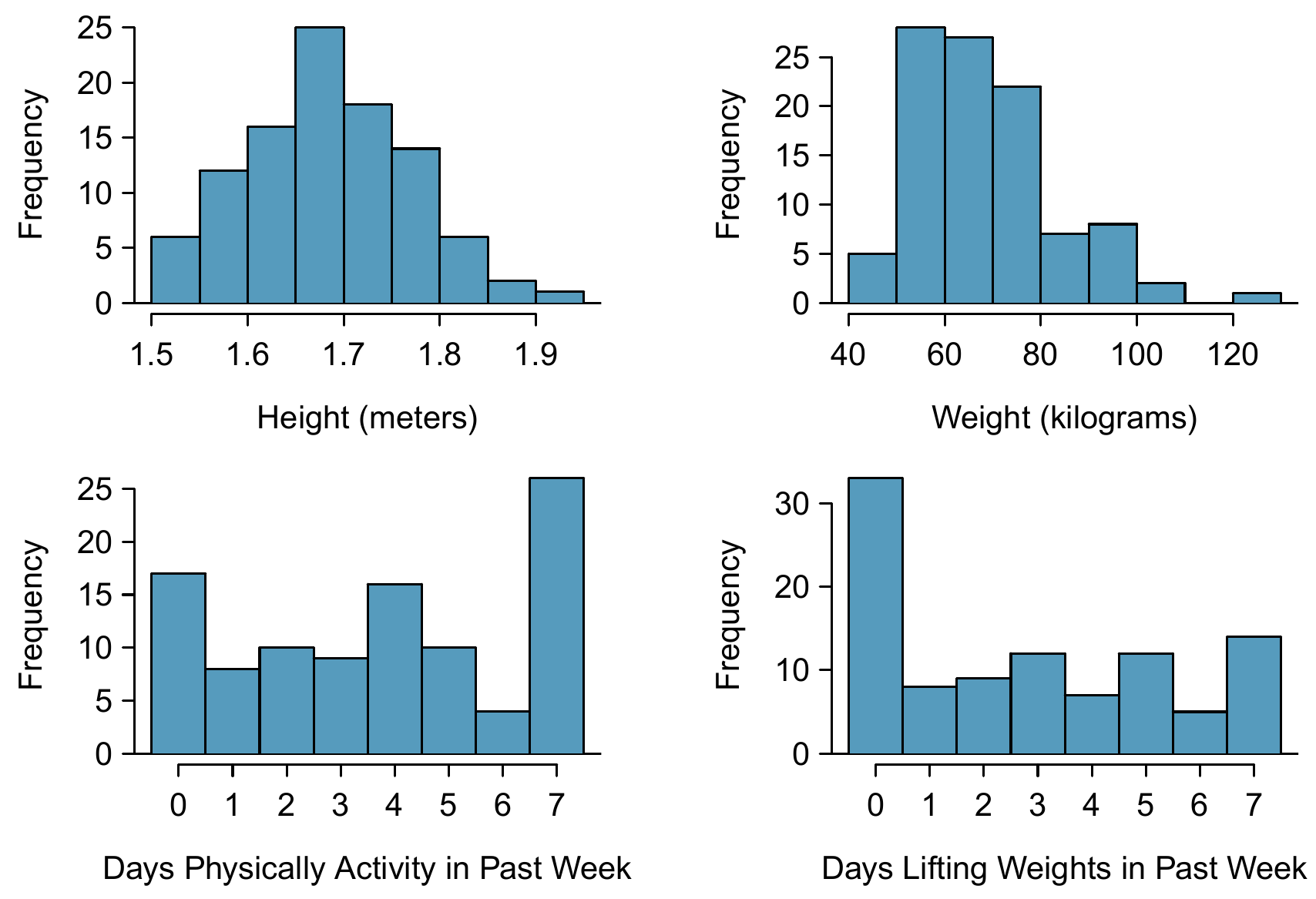
$Histograms of $\texttt{height}$, $\texttt{weight}$, $\texttt{activity}$, and $\texttt{lifting}$ for the sample YRBSS data. The $\texttt{height}$ distribution is approximately symmetric, $\texttt{weight}$ is moderately skewed to the right, $\texttt{activity}$ is bimodal or multimodal (with unclear skew), and $\texttt{lifting}$ is strongly right skewed.$

Figure 9.1: Histograms of $\texttt{height}$, $\texttt{weight}$, $\texttt{activity}$, and $\texttt{lifting}$ for the sample YRBSS data. The $\texttt{height}$ distribution is approximately symmetric, $\texttt{weight}$ is moderately skewed to the right, $\texttt{activity}$ is bimodal or multimodal (with unclear skew), and $\texttt{lifting}$ is strongly right skewed.

9.1 Variability in Estimates

We would like to estimate four features of the high schoolers in YRBSS using the sample.

What is the average height of the YRBSS high schoolers?
What is the average weight of the YRBSS high schoolers?
On average, how many days per week are YRBSS high schoolers physically active?
On average, how many days per week do YRBSS high schoolers do weight training?

While we focus on the mean in this chapter, questions regarding variation are often just as important in practice. For instance, if students are either very active or almost entirely inactive (the distribution is bimodal), we might try different strategies to promote a healthy lifestyle among students than if all high schoolers were already somewhat active.

9.1.1 Point estimates

We want to estimate the population mean based on the sample. The most intuitive way to go about doing this is to simply take the sample mean. That is, to estimate the average height of all YRBSS students, take the average height for the sample: \[ \bar{x}_{height} = \frac{1.50 + 1.78 + \dots + 1.70}{100} = 1.697 \]

The sample mean $\bar{x} = 1.697$ meters (5 feet, 6.8 inches) is called a point estimate of the population mean: if we can only choose one value to estimate the population mean, this is our best guess. Suppose we take a new sample of 100 people and recompute the mean; we will probably not get the exact same answer that we got using the yrbss_samp data set. Estimates generally vary from one sample to another, and this sampling variation suggests our estimate may be close, but it will not be exactly equal to the parameter.

We can also estimate the average weight of YRBSS respondents by examining the sample mean of $\texttt{weight}$ (in kg), and average number of days physically active in a~week:

\[ \begin{aligned} \bar{x}_{weight} &= \frac{52.6 + 74.8 + \dots + 55.8}{100}= 68.89\\ \bar{x}_{active} &= \frac{0 + 7 + \dots + 1}{100}= 3.75 \end{aligned} \] The average weight is 68.89 kilograms.

What about generating point estimates of other population parameters, such as the population median or population standard deviation? Once again we might estimate parameters based on sample statistics, as shown in Table 9.4. For example, the population standard deviation of $\texttt{active}$ using the sample standard deviation, 2.56 days.

Table 9.4: Estimates for $\texttt{active}$ variable.
$\texttt{active}$	estimate	parameter
mean	3.75	3.90
median	4.00	4.00
st. deviation	2.556	2.564

9.1.2 Point estimates are not exact

Estimates are usually not exactly equal to the truth, but they get better as more data become available. We can see this by plotting a running mean from yrbss_samp. A running mean is a sequence of means, where each mean uses one more observation in its calculation than the mean directly before it in the sequence. For example, the second mean in the sequence is the average of the first two observations and the third in the sequence is the average of the first three. The running mean for the $\texttt{active}$ variable in the yrbss_samp is shown in Figure 9.2, and it approaches the true population average, 3.90~days, as more data become available.

The mean computed after adding each individual to the sample. The mean tends to approach the true population average as more data become available.

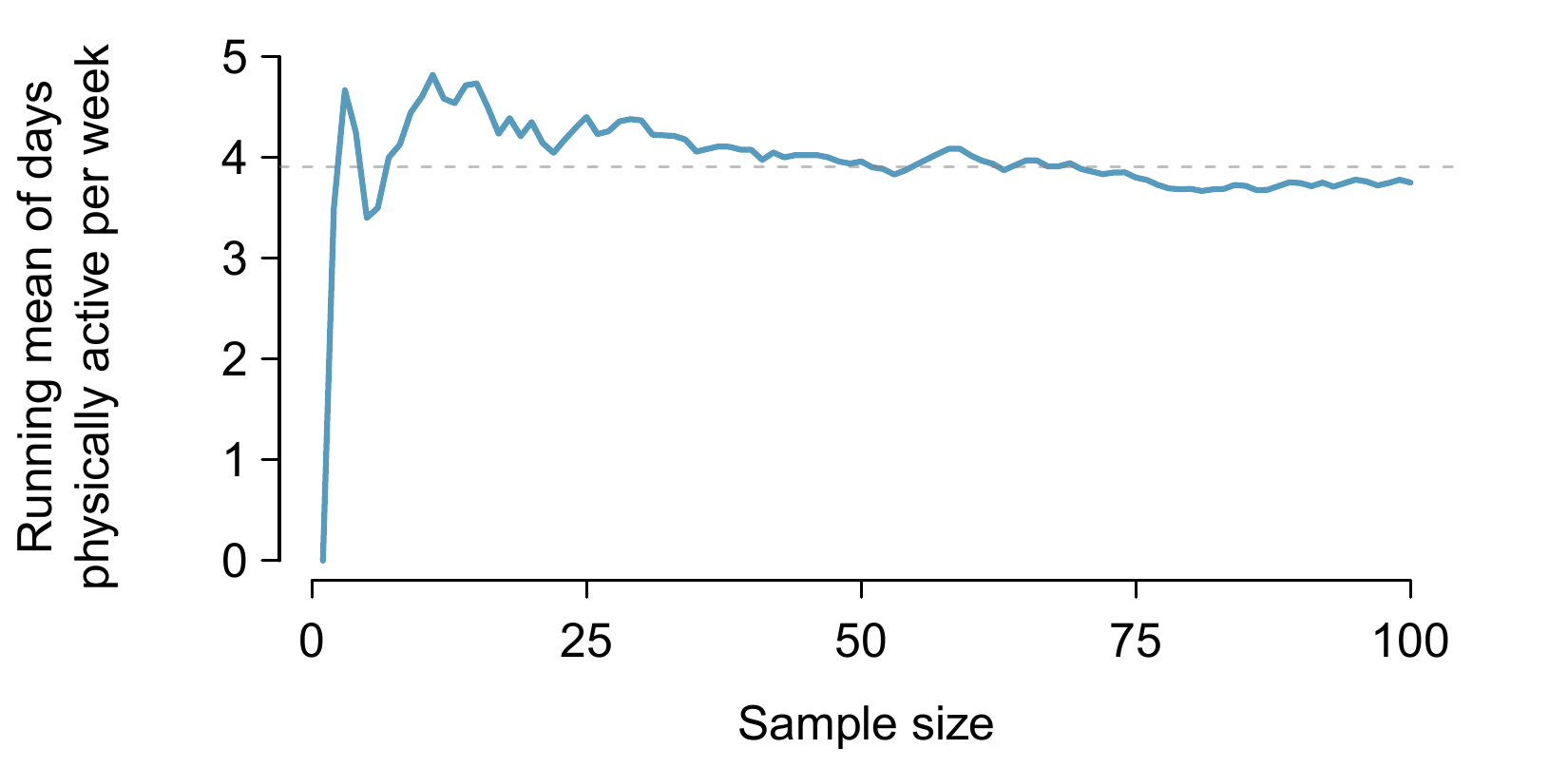
Figure 9.2: The mean computed after adding each individual to the sample. The mean tends to approach the true population average as more data become available.

Sample point estimates only approximate the population parameter, and they vary from one sample to another. If we took another simple random sample of the YRBSS students, we would find that the sample mean for the number of days active would be a little different. It will be useful to quantify how variable an estimate is from one sample to another. If this variability is small (i.e. the sample mean doesn’t change much from one sample to another) then that estimate is probably very accurate. If it varies widely from one sample to another, then we should not expect our estimate to be very good.

9.1.3 Standard error of the mean

From the random sample represented in yrbss_samp, we guessed the average number of days a YRBSS student is physically active is 3.75~days. Suppose we take another random sample of 100 individuals and take its mean: 3.22~days. Suppose we took another (3.67~days) and another (4.10~days), and so on. If we do this many many times – which we can do only because we have all YRBSS students – we can build up a sampling distribution for the sample mean when the sample size is 100, shown in Figure 9.3.

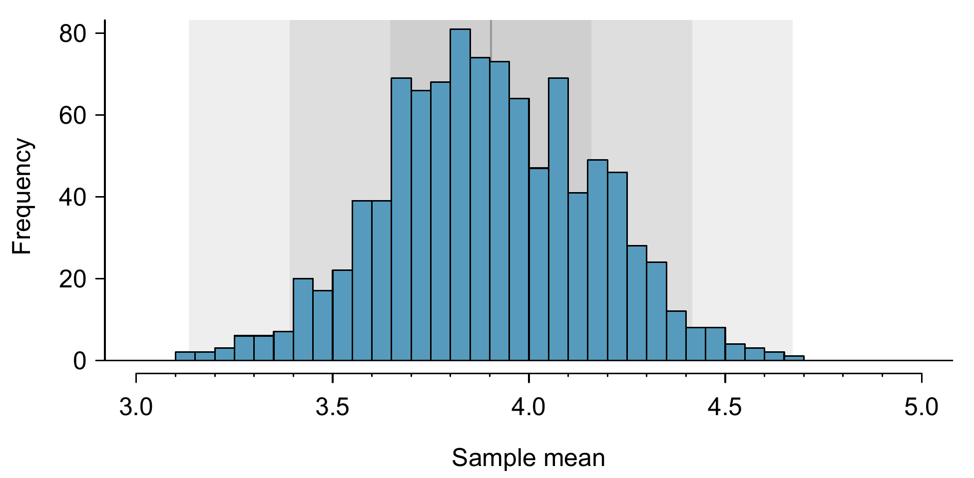
Figure 9.3: A histogram of 1000 sample means for number of days physically active per week, where the samples are of size $n=100$.

Definition 9.1 (Sampling distribution) The sampling distribution represents the distribution of the point estimates based on samples of a fixed size from a certain population. It is useful to think of a particular point estimate as being drawn from such a distribution. Understanding the concept of a sampling distribution is central to understanding statistical inference.

The sampling distribution shown in Figure 9.3 is unimodal and approximately symmetric. It is also centred exactly at the true population mean: $\mu=3.90$. Intuitively, this makes sense. The sample means should tend to “fall around” the population mean.

We can see that the sample mean has some variability around the population mean, which can be quantified using the standard deviation of this distribution of sample means: $\sigma_{\bar{x}} = 0.26$. The standard deviation of the sample mean tells us how far the typical estimate is away from the actual population mean, 3.90~days. It also describes the typical error of the point estimate, and for this reason we usually call this standard deviation the standard error (SE).

Definition 9.2 (Standard error of an estimate) The standard deviation associated with an estimate is called the standard error. It describes the typical error or uncertainty associated with the estimate.

When considering the case of the point estimate $\bar{x}$, there is one problem: there is no obvious way to estimate its standard error from a single sample. However, statistical theory provides a helpful tool to address this issue.

Guided Practice9.1
(a) Would you rather use a small sample or a large sample when estimating a parameter? Why?
(b) Using your reasoning from (a), would you expect a point estimate based on a small sample to have smaller or larger standard error than a point estimate based on a larger sample?⁹¹

In the sample of 100 students, the standard error of the sample mean is equal to the population standard deviation divided by the square root of the sample size: \[ SE_{\bar{x}} = \sigma_{\bar{x}} = \frac{\sigma_{x}}{\sqrt{n}} = \frac{2.6}{\sqrt{100}} = 0.26 \] where $\sigma_{x}$ is the standard deviation of the individual observations. This is no coincidence. We can show mathematically that this equation is correct when the observations are independent.

Definition 9.3 (Computing SE for the sample mean) Given $n$ independent observations from a population with standard deviation $\sigma$, the standard error of the sample mean is equal to \[ SE = \frac{\sigma}{\sqrt{n}} \tag{9.1} \] A reliable method to ensure sample observations are independent is to conduct a simple random sample consisting of less than 10% of the population.

There is one subtle issue in Equation (9.1): the population standard deviation is typically unknown. You might have already guessed how to resolve this problem: we can use the point estimate of the standard deviation from the sample. This estimate tends to be sufficiently good when the sample size is at least 30 and the population distribution is not strongly skewed.

Thus, we often just use the sample standard deviation $s$ instead of $\sigma$. When the sample size is smaller than 30, we will need to use a method to account for extra uncertainty in the standard error. If the skew condition is not met, a larger sample is needed to compensate for the extra skew. These topics are further discussed in Section 9.4.

Guided Practice9.2
In the sample of 100 students, the standard deviation of student heights is $s_{height} = 0.088$ meters. In this case, we can confirm that the observations are independent by checking that the data come from a simple random sample consisting of less than 10% of the population.
(a) What is the standard error of the sample mean, $\bar{x}_{height} = 1.70$ meters?
(b) Would you be surprised if someone told you the average height of all YRBSS respondents was actually 1.69~meters?⁹²

Guided Practice9.3
(a) Would you be more trusting of a sample that has 100 observations or 400 observations?
(b) We want to show mathematically that our estimate tends to be better when the sample size is larger. If the standard deviation of the individual observations is 10, what is our estimate of the standard error when the sample size is 100? What about when it is 400?
(c) Explain how your answer to part (b) mathematically justifies your intuition in part (a).⁹³

9.1.4 Basic properties of point estimates

We achieved three goals in this section. First, we determined that point estimates from a sample may be used to estimate population parameters. We also determined that these point estimates are not exact: they vary from one sample to another. Lastly, we quantified the uncertainty of the sample mean using what we call the standard error, mathematically represented in Equation (9.1). While we could also quantify the standard error for other estimates – such as the median, standard deviation, or any other number of statistics – these are beyond the scope of the current course.

9.2 Confidence Intervals

A point estimate provides a single plausible value for a parameter. However, a point estimate is rarely perfect; usually there is some error in the estimate. Instead of supplying just a point estimate of a parameter, a next logical step would be to provide a plausible range of values for the parameter.

9.2.1 Capturing the population parameter

A plausible range of values for the population parameter is called a confidence interval.

Using only a point estimate is like fishing in a murky lake with a spear, and using a confidence interval is like fishing with a net. We can throw a spear where we saw a fish, but we will probably miss. On the other hand, if we toss a net in that area, we have a good chance of catching the fish.

If we report a point estimate, we probably will not hit the exact population parameter. On the other hand, if we report a range of plausible values – a confidence interval – we have a good shot at capturing the parameter.

Guided Practice9.4
If we want to be very certain we capture the population parameter, should we use a wider interval or a smaller interval?⁹⁴

9.2.2 An approximate 95% confidence interval

Our point estimate is the most plausible value of the parameter, so it makes sense to build the confidence interval around the point estimate. The standard error, which is a measure of the uncertainty associated with the point estimate, provides a guide for how large we should make the confidence interval.

The standard error represents the standard deviation associated with the estimate, and roughly 95% of the time the estimate will be within 2 standard errors of the parameter. If~the interval spreads out 2 standard errors from the point estimate, we can be roughly 95% that we have captured the true parameter: \[ \text{point estimate}\ \pm\ 2\times SE \tag{9.2} \] But what does “95% confident” mean? Suppose we took many samples and built a confidence interval from each sample using Equation (9.2). Then about 95% of those intervals would contain the actual mean, $\mu$. Figure 9.4 shows this process with 25 samples, where 24 of the resulting confidence intervals contain the average number of days per week that YRBSS students are physically active, $\mu=3.90$ days, and one interval does not.

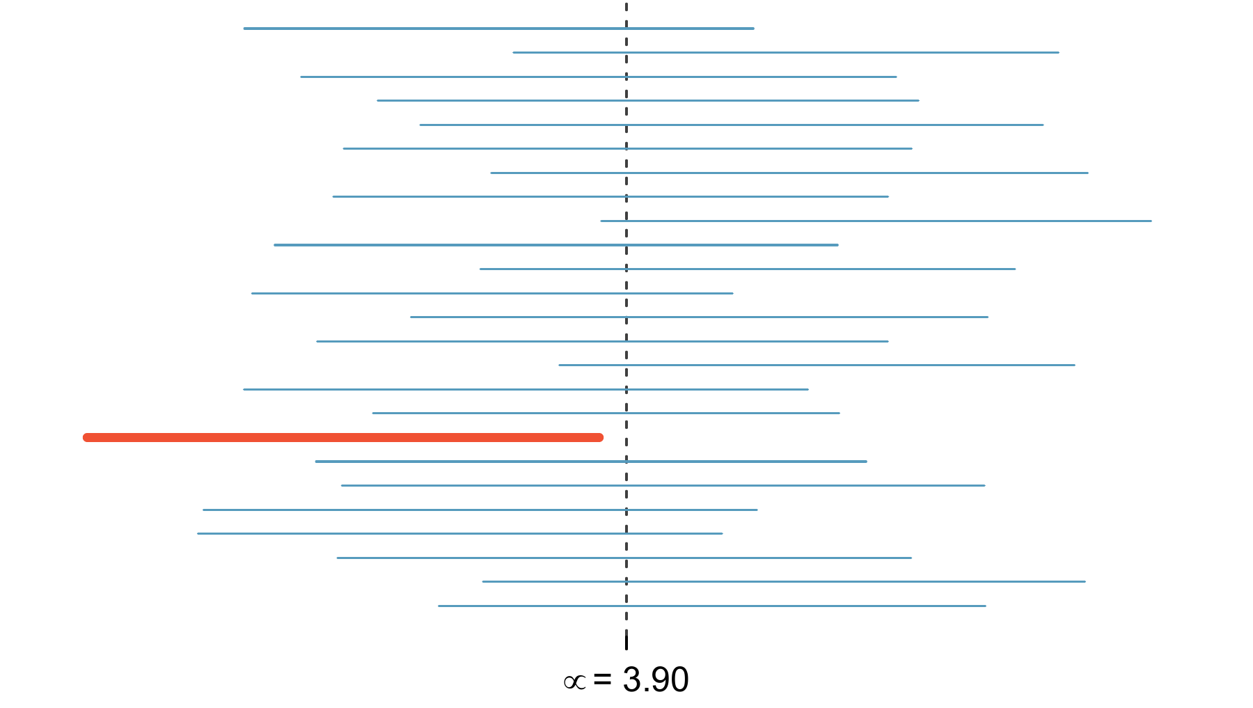
$Twenty-five samples of size $n=100$ were taken from yrbss. For~each sample, a confidence interval was created to try to capture the average number of days per week that students are physically active. Only 1 of these 25 intervals did not capture the true mean, $\mu = 3.90$ days.$

Figure 9.4: Twenty-five samples of size $n=100$ were taken from yrbss. For~each sample, a confidence interval was created to try to capture the average number of days per week that students are physically active. Only 1 of these 25 intervals did not capture the true mean, $\mu = 3.90$ days.

Guided Practice9.5
In Figure 9.4, one interval does not contain 3.90 minutes. Does this imply that the mean cannot be 3.90?⁹⁵

The rule where about 95% of observations are within 2 standard deviations of the mean is only approximately true. However, it holds very well for the normal distribution. As we will soon see, the mean tends to be normally distributed when the sample size is sufficiently large.

Example 9.1
The sample mean of days active per week from yrbss_samp is 3.75~days. The standard error, as estimated using the sample standard deviation, is $SE=\frac{2.6}{\sqrt{100}} = 0.26$~days. (The population SD is unknown in most applications, so we use the sample SD here.) Calculate an approximate 95% confidence interval for the average days active per week for all YRBSS students.
We apply Equation (9.2): \[ 3.75\ \pm\ 2 \times 0.26 \quad \rightarrow \quad (3.23, 4.27) \]
Based on these data, we are about 95% confident that the average days active per week for all YRBSS students was larger than 3.23 but less than 4.27 days. Our interval extends out 2 standard errors from the point estimate, $\bar{x}_{active}$.

Guided Practice9.6
The sample data suggest the average YRBSS student height is $\bar{x}_{height} = 1.697$ meters with a standard error of 0.0088 meters (estimated using the sample standard deviation, 0.088 meters). What is an approximate 95% confidence interval for the average height of all of the YRBSS students?^[Apply Equation (9.2): $1.697 \ \pm \ 2\times 0.0088 \rightarrow (1.6794, 1.7146)$. We interpret this interval as follows: We are about 95% confident the average height of all YRBSS students was between 1.6794 and 1.7146 meters.}

9.2.3 The sampling distribution for the mean

In Section 9.1.3, we introduced a sampling distribution for $\bar{x}$, the average days physically active per week for samples of size 100. We examined this distribution earlier in Figure 9.3. Now we’ll take 100,000 samples, calculate the mean of each, and plot them in a histogram to get an especially accurate depiction of the sampling distribution. This histogram is shown in the left panel of Figure 9.5.

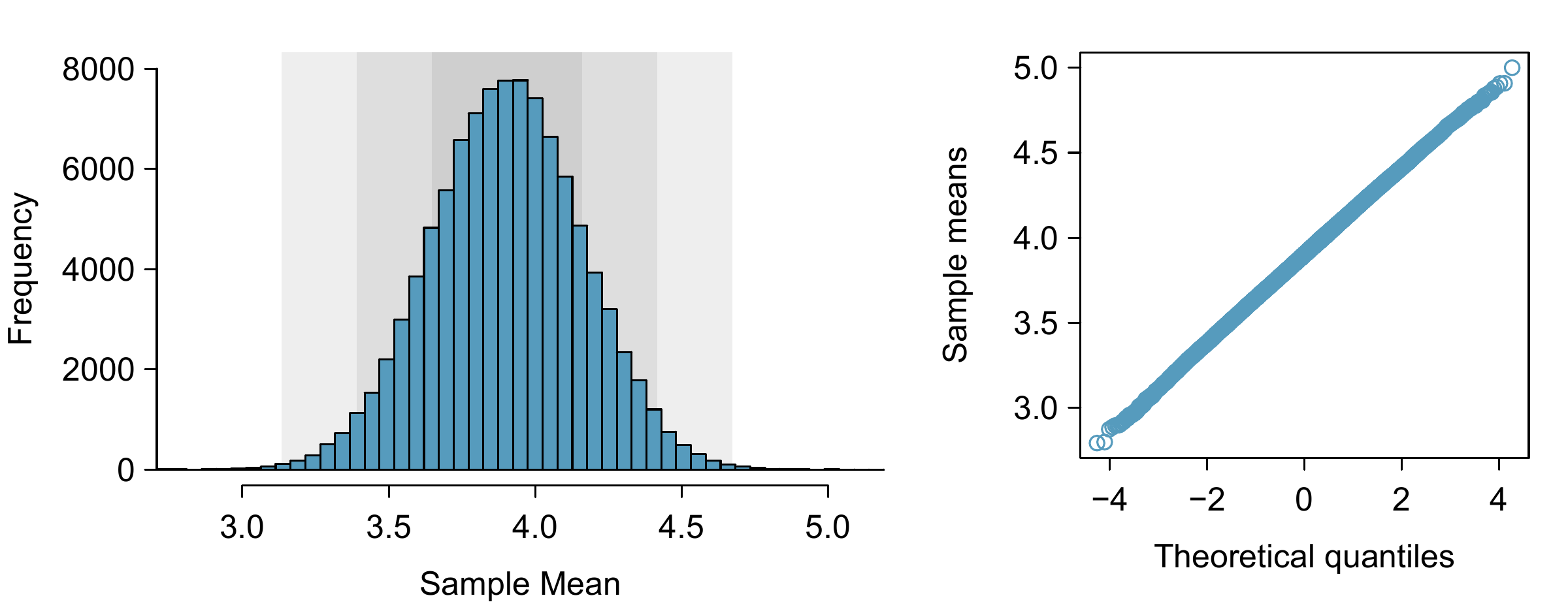
The left panel shows a histogram of the sample means for 100,000 different random samples. The right panel shows a normal probability plot of those sample means.

Figure 9.5: The left panel shows a histogram of the sample means for 100,000 different random samples. The right panel shows a normal probability plot of those sample means.

Does this distribution look familiar? Hopefully so! The distribution of sample means closely resembles the normal distribution. A normal probability plot of these sample means is shown in the right panel of Figure 9.5. Because all of the points closely fall around a straight line, we can conclude the distribution of sample means is nearly normal. This result can be explained by the Central Limit Theorem.

Definition 9.4 (Central Limit Theorem, informal description) If a sample consists of at least 30 independent observations and the data are not strongly skewed, then the distribution of the sample mean is well approximated by a normal model.

We will apply this informal version of the Central Limit Theorem for now, and discuss its details further in Section 9.4.

The choice of using 2 standard errors in Equation (9.2) was based on our general guideline that roughly 95% of the time, observations are within two standard deviations of the mean. Under the normal model, we can make this more accurate by using 1.96 in place of 2.

\[ \text{point estimate}\ \pm\ 1.96\times SE \tag{9.3} \] If a point estimate, such as $\bar{x}$, is associated with a normal model and standard error $SE$, then we use this more precise 95% confidence interval.

9.2.4 Interpreting confidence intervals

A careful eye might have observed the somewhat awkward language used to describe confidence intervals. Correct interpretation:

We are XX% confident that the population parameter is between…

Incorrect language might try to describe the confidence interval as capturing the population parameter with a certain probability. This is a common error: while it might be useful to think of it as a probability, the confidence level only quantifies how plausible it is that the parameter is in the interval.

Another important consideration of confidence intervals is that they only try to capture the population parameter. A confidence interval says nothing about the confidence of capturing individual observations, a proportion of the observations, or about capturing point estimates. Confidence intervals only attempt to capture population parameters.

9.3 Hypothesis Testing

Are students lifting weights or performing other strength training exercises more or less often than they have in the past? We’ll compare data from students from the 2011 YRBSS survey to our sample of 100 students from the 2013 YRBSS survey.

We’ll also consider sleep behavior. A recent study found that college students average about 7~hours of sleep per night.⁹⁶ However, researchers at a rural college are interested in showing that their students sleep longer than seven hours on average. We investigate this topic in Section 9.3.3.

9.3.1 Hypothesis testing framework

Students from the 2011 YRBSS lifted weights (or performed other strength training exercises) 3.09~days per week on average. We want to determine if the yrbss_samp data set provides strong evidence that YRBSS students selected in 2013 are lifting more or less than the 2011 YRBSS students, versus the other possibility that there has been no change.⁹⁷ We simplify these three options into two competing hypotheses:

$H_0$: The average days per week that YRBSS students lifted weights was the same for 2011 and 2013.
$H_A$: The average days per week that YRBSS students lifted weights was different for 2013 than in 2011.

We call $H_0$ the null hypothesis and $H_A$ the alternative hypothesis.

Definition 9.5 (Null and alternative hypotheses) The null hypothesis ($H_0$) often represents either a sceptical perspective or a claim to be tested. The alternative hypothesis ($H_A$) represents an alternative claim under consideration and is often represented by a range of possible parameter values.

The null hypothesis often represents a sceptical position or a perspective of no difference. The alternative hypothesis often represents a new perspective, such as the possibility that there has been a change.

Remark (Hypothesis testing framework). The sceptic will not reject the null hypothesis ($H_0$), unless the evidence in favour of the alternative hypothesis ($H_A$) is so strong that she rejects $H_0$ in favour of $H_A$.

The hypothesis testing framework is a very general tool, and we often use it without a second thought. If a person makes a somewhat unbelievable claim, we are initially sceptical. However, if there is sufficient evidence that supports the claim, we set aside our scepticism and reject the null hypothesis in favour of the alternative. The hallmarks of hypothesis testing are also found in the court system.

Guided Practice9.7
A court considers two possible claims about a defendant: she is either innocent or guilty. If we set these claims up in a hypothesis framework, which would be the null hypothesis and which the alternative?⁹⁸

Jurors examine the evidence to see whether it convincingly shows a defendant is guilty. Even if the jurors leave unconvinced of guilt beyond a reasonable doubt, this does not mean they believe the defendant is innocent. This is also the case with hypothesis testing: even if we fail to reject the null hypothesis, we typically do not accept the null hypothesis as true. Failing to find strong evidence for the alternative hypothesis is not equivalent to accepting the null hypothesis.

In the example with the YRBSS, the null hypothesis represents no difference in the average days per week of weight lifting in 2011 and 2013. The alternative hypothesis represents something new or more interesting: there was a difference, either an increase or a decrease. These hypotheses can be described in mathematical notation using $\mu_{13}$ as the average days of weight lifting for 2013:

$H_0$: $\mu_{13} = 3.09$
$H_A$: $\mu_{13} \neq 3.09$

where 3.09 is the average number of days per week that students from the 2011 YRBSS lifted weights. Using the mathematical notation, the hypotheses can more easily be evaluated using statistical tools. We call 3.09 the null value since it represents the value of the parameter if the null hypothesis is true.

9.3.2 Decision errors

Hypothesis tests are not flawless, since we can make a wrong decision in statistical hypothesis tests based on the data. For example, in the court system innocent people are sometimes wrongly convicted and the guilty sometimes walk free. However, the difference is that in statistical hypothesis tests, we have the tools necessary to quantify how often we make such errors.

There are two competing hypotheses: the null and the alternative. In a hypothesis test, we make a statement about which one might be true, but we might choose incorrectly. There are four possible scenarios, which are summarized in Table 9.5.

Table 9.5: Four different scenarios for hypothesis tests.
	Conclusion:do no reject $H_0$	Conclusion: reject $H_0$ in favour of $H_A$
$H_0$ true	okay	Type 1 error
	$(1-\alpha)$	$(\alpha)$
$H_A$ true	Type 2 error	okay
	$(\beta)$	$(1-\beta)$

A Type 1 Error is rejecting the null hypothesis when $H_0$ is actually true. A Type 2 Error is failing to reject the null hypothesis when the alternative is actually true.

Guided Practice9.8
In a court, the defendant is either innocent ($H_0$) or guilty ($H_A$).

What does a Type 1 Error represent in this context?
What does a Type 2 Error represent? Table 9.5 may be useful.⁹⁹

Guided Practice9.9

How could we reduce the Type 1 Error rate in courts?
What influence would this have on the Type 2 Error rate?¹⁰⁰

Guided Practice9.10

How could we reduce the Type 2 Error rate in courts?
What influence would this have on the Type 1 Error rate?¹⁰¹

Exercises 9.8-9.10 provide an important lesson: if we reduce how often we make one type of error, we generally make more of the other type.

Hypothesis testing is built around rejecting or failing to reject the null hypothesis. That is, we do not reject $H_0$ unless we have strong evidence. But what precisely does strong evidence mean? As a general rule of thumb, for those cases where the null hypothesis is actually true, we do not want to incorrectly reject $H_0$ more than 5% of the time. This corresponds to a significance level of 0.05. We often write the significance level using $\alpha$ (the Greek letter ): $\alpha = 0.05$.

If we use a 95% confidence interval to evaluate a hypothesis test where the null hypothesis is true, we will make an error whenever the point estimate is at least 1.96 standard errors away from the population parameter. This happens about 5% of the time (2.5% in each tail). Similarly, using a 99% confidence interval to evaluate a hypothesis is equivalent to a significance level of $\alpha = 0.01$.

A confidence interval is, in one sense, simplistic in the world of hypothesis tests. Consider the following two scenarios:

The null value (the parameter value under the null hypothesis) is in the 95% confidence interval but just barely, so we would not reject $H_0$. However, we might like to somehow say, quantitatively, that it was a close decision.
The null value is very far outside of the interval, so we reject $H_0$. However, we want to communicate that, not only did we reject the null hypothesis, but it wasn’t even close. Such a case is depicted in Figure 9.6.

In Section 9.3.3, we introduce a tool called the p-value that will be helpful in these cases. The p-value method also extends to hypothesis tests where confidence intervals cannot be easily constructed or applied.

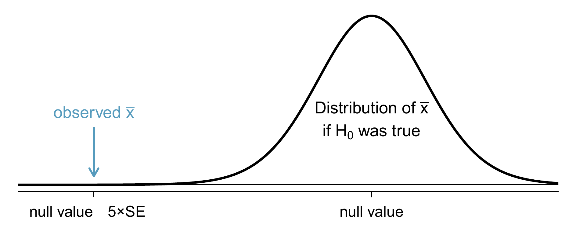
Figure 9.6: It would be helpful to quantify the strength of the evidence against the null hypothesis. In this case, the evidence is extremely strong.

9.3.3 Formal testing using p-values

The p-value is a way of quantifying the strength of the evidence against the null hypothesis and in favour of the alternative. Formally the p-value is a conditional probability.

Definition 9.6 (p-value) The p-value is the probability of observing data at least as favourable to the alternative hypothesis as our current data set, if the null hypothesis is true. We typically use a summary statistic of the data, in this chapter the sample mean, to help compute the p-value and evaluate the hypotheses.

Guided Practice9.11
A poll by the National Sleep Foundation found that college students average about 7 hours of sleep per night. Researchers at a rural school are interested in showing that students at their school sleep longer than seven hours on average, and they would like to demonstrate this using a sample of students. What would be an appropriate sceptical position for this research?¹⁰²

We can set up the null hypothesis for this test as a sceptical perspective: the students at this school average 7 hours of sleep per night. The alternative hypothesis takes a new form reflecting the interests of the research: the students average more than 7 hours of sleep. We can write these hypotheses as

$H_0$: $\mu = 7$.
$H_A$: $\mu > 7$.

Using $\mu > 7$ as the alternative is an example of a one-sided hypothesis test. In this investigation, there is no apparent interest in learning whether the mean is less than 7 hours.¹⁰³ Earlier we encountered a two-sided hypothesis where we looked for any clear difference, greater than or less than the null value.

Always use a two-sided test unless it was made clear prior to data collection that the test should be one-sided. Switching a two-sided test to a one-sided test after observing the data is dangerous because it can inflate the Type 1 Error rate.

Remark (One-sided and two-sided tests). When you are interested in checking for an increase or a decrease, but not both, use a one-sided test. When you are interested in any difference from the null value_–an increase or decrease_–then the test should be two-sided.

Remark (Always write the null hypothesis as an equality). We will find it most useful if we always list the null hypothesis as an equality (e.g. $\mu = 7$) while the alternative always uses an inequality (e.g. $\mu\neq7$, $\mu>7$, or $\mu<7$).

The researchers at the rural school conducted a simple random sample of $n=110$ students on campus. They found that these students averaged 7.42 hours of sleep and the standard deviation of the amount of sleep for the students was 1.75 hours. A histogram of the sample is shown in Figure 9.7.

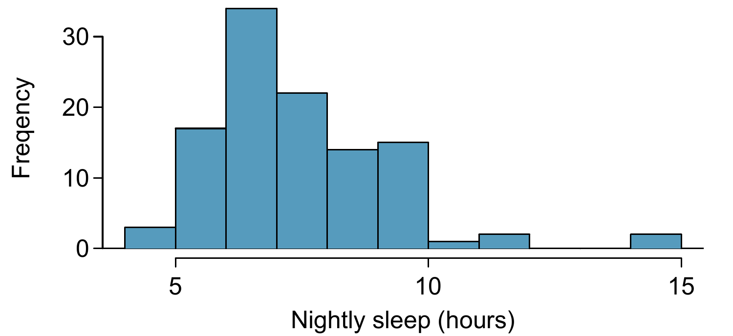
Figure 9.7: Distribution of a night of sleep for 110 college students. These data are strongly skewed.

Before we can use a normal model for the sample mean or compute the standard error of the sample mean, we must verify conditions.

Because this is a simple random sample from less than 10% of the student body, the observations are independent.
The sample size in the sleep study is sufficiently large since it is greater than 30.
The data show strong skew in Figure 9.7 and the presence of a couple of outliers. This skew and the outliers are acceptable for a sample size of $n=110$. With these conditions verified, the normal model can be safely applied to $\bar{x}$ and we can reasonably calculate the standard error.

Guided Practice9.12
In the sleep study, the sample standard deviation was 1.75 hours and the sample size is 110. Calculate the standard error of $\bar{x}$.¹⁰⁴

The hypothesis test for the sleep study will be evaluated using a significance level of $\alpha = 0.05$. We want to consider the data under the scenario that the null hypothesis is true. In this case, the sample mean is from a distribution that is nearly normal and has mean 7 and standard deviation of about $SE_{\bar{x}} = 0.17$. Such a distribution is shown in Figure 9.8.

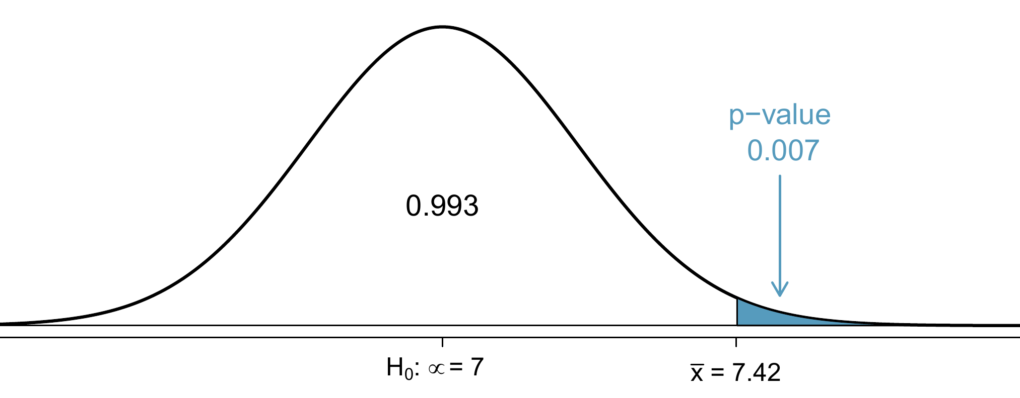
$If the null hypothesis is true, then the sample mean $\bar{x}$ came from this nearly normal distribution. The right tail describes the probability of observing such a large sample mean if the null hypothesis is true.$

Figure 9.8: If the null hypothesis is true, then the sample mean $\bar{x}$ came from this nearly normal distribution. The right tail describes the probability of observing such a large sample mean if the null hypothesis is true.

The shaded tail in Figure 9.8 represents the chance of observing such a large mean, conditional on the null hypothesis being true. That is, the shaded tail represents the $\mbox{p-value}$. We shade all means larger than our sample mean, $\bar{x} = 7.42$, because they are more favourable to the alternative hypothesis than the observed mean.

We compute the p-value by finding the tail area of this normal distribution. First compute the Z-score of the sample mean, $\bar{x} = 7.42$: \[ Z = \frac{\bar{x} - \text{null value}}{SE_{\bar{x}}} = \frac{7.42 - 7}{0.17} = 2.47 \] Using the normal probability table, the lower unshaded area is found to be 0.993. Thus the shaded area is $1-0.993 = 0.007$. If the null hypothesis is true, the probability of observing a sample mean at least as large as 7.42 hours for a sample of 110 students is only 0.007. That is, if the null hypothesis is true, we would not often see such a large mean.

We evaluate the hypotheses by comparing the p-value to the significance level. Because the p-value is less than the significance level (p-value $=0.007 < 0.05=\alpha$), we reject the null hypothesis. What we observed is so unusual with respect to the null hypothesis that it casts serious doubt on $H_0$ and provides strong evidence favouring $H_A$.

Definition 9.7 (p-value as a tool in hypothesis testing) The smaller the p-value, the stronger the data favour $H_A$ over $H_0$. A small p-value (usually $<0.05$) corresponds to sufficient evidence to reject $H_0$ in favour of $H_A$.

Remark (It is useful to first draw a picture to find the p-value). It is useful to draw a picture of the distribution of $\bar{x}$ as though $H_0$ was true (i.e. $\mu$ equals the null value), and shade the region (or regions) of sample means that are at least as favourable to the alternative hypothesis. These shaded regions represent the p-value.}

The ideas below review the process of evaluating hypothesis tests with p-values:

The null hypothesis represents a sceptic’s position or a position of no difference. We reject this position only if the evidence strongly favours $H_A$.
A small p-value means that if the null hypothesis is true, there is a low probability of seeing a point estimate at least as extreme as the one we saw. We interpret this as strong evidence in favour of the alternative.
We reject the null hypothesis if the p-value is smaller than the significance level, $\alpha$, which is usually 0.05. Otherwise, we fail to reject $H_0$.
We should always state the conclusion of the hypothesis test in plain language so non-statisticians can also understand the results.

The p-value is constructed in such a way that we can directly compare it to the significance level ($\alpha$) to determine whether or not to reject $H_0$. This method ensures that the Type 1 Error rate does not exceed the significance level standard.

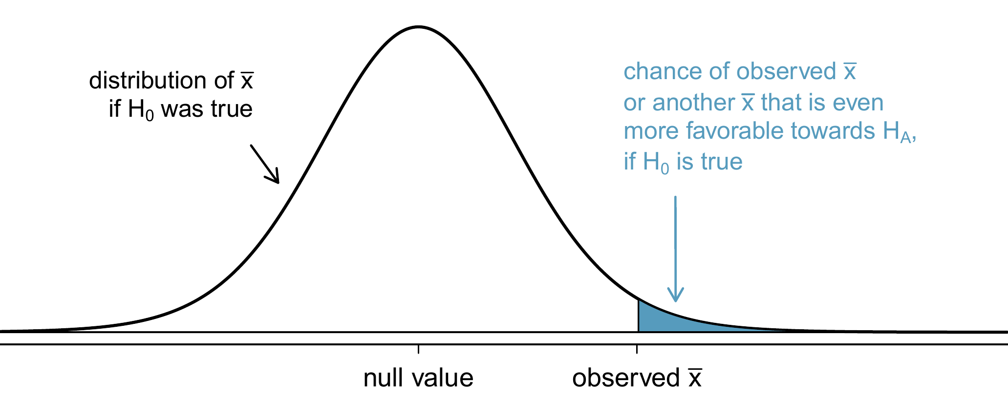
$To identify the p-value, the distribution of the sample mean is considered as if the null hypothesis was true. Then the p-value is defined and computed as the probability of the observed $\bar{x}$ or an $\bar{x}$ even more favourable to $H_A$ under this distribution.$

Figure 9.9: To identify the p-value, the distribution of the sample mean is considered as if the null hypothesis was true. Then the p-value is defined and computed as the probability of the observed $\bar{x}$ or an $\bar{x}$ even more favourable to $H_A$ under this distribution.

Guided Practice9.13
If the null hypothesis is true, how often should the p-value be less than 0.05?¹⁰⁵

Guided Practice9.14
Suppose we had used a significance level of 0.01 in the sleep study. Would the evidence have been strong enough to reject the null hypothesis? (The p-value was 0.007.) What if the significance level was $\alpha = 0.001$?¹⁰⁶

Guided Practice9.15
Ebay might be interested in showing that buyers on its site tend to pay less than they would for the corresponding new item on Amazon. We’ll research this topic for one particular product: a video game called Mario Kart for the Nintendo Wii. During early October 2009, Amazon sold this game for $46.99. Set up an appropriate (one-sided!) hypothesis test to check the claim that Ebay buyers pay less during auctions at this same time.¹⁰⁷

Guided Practice9.16
During early October 2009, 52 Ebay auctions were recorded for .¹⁰⁸ The total prices for the auctions are presented using a histogram in Figure 9.10, and we may like to apply the normal model to the sample mean. Check the three conditions required for applying the normal model:

independence,
at least 30 observations, and
the data are not strongly skewed.¹⁰⁹

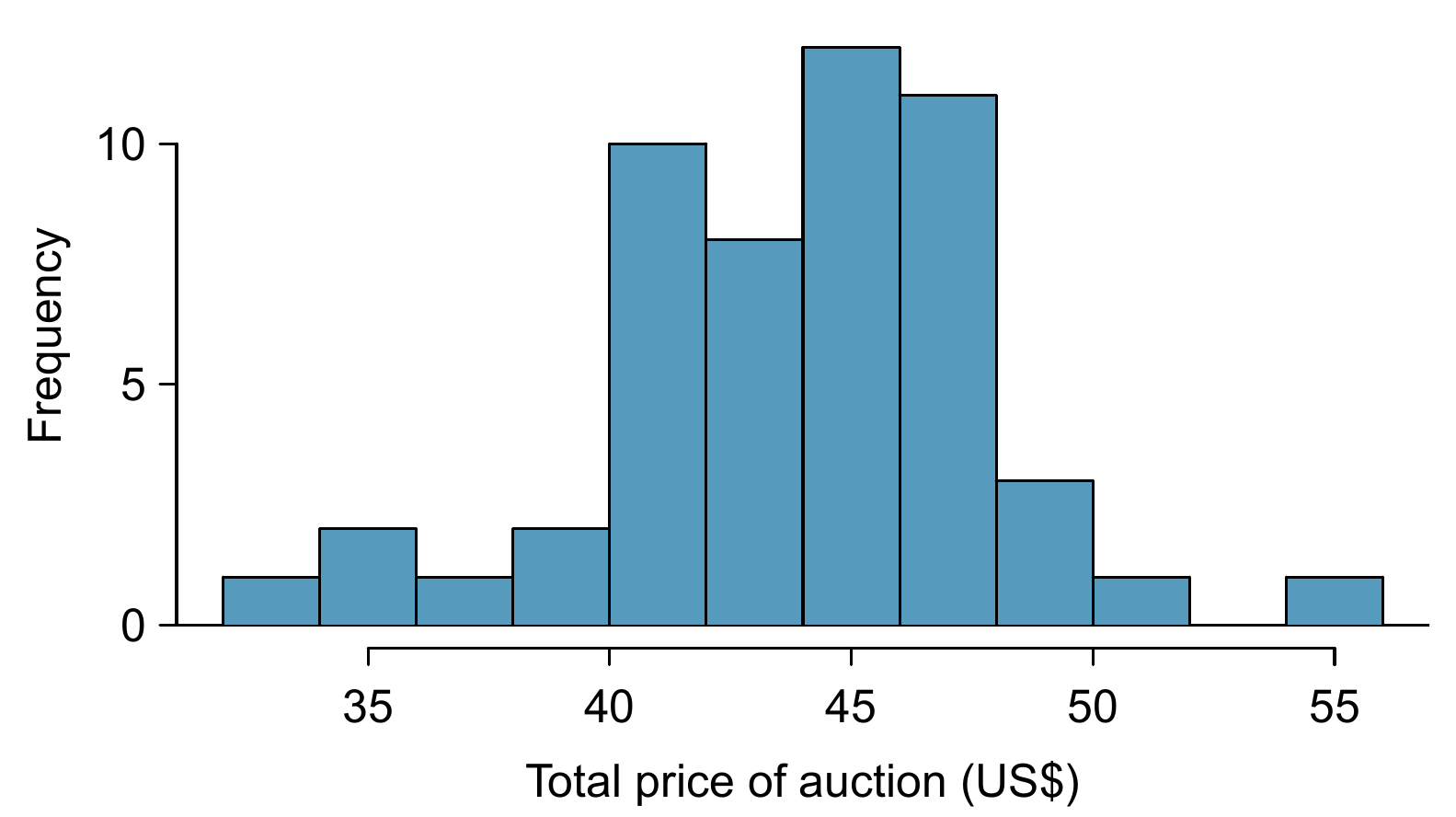
Figure 9.10: A histogram of the total auction prices for 52 Ebay auctions.

Example 9.2
The average sale price of the 52 Ebay auctions for Wii Mario Kart was $44.17 with a standard deviation of $4.15. Does this provide sufficient evidence to reject the null hypothesis in Guided Practice 9.15? Use a significance level of $\alpha = 0.01$.

The hypotheses were set up and the conditions were checked in Exercises 9.15 and 9.16. The next step is to find the standard error of the sample mean and produce a sketch to help find the p-value. \[ SE_{\bar{x}} = s/\sqrt{n} = 4.15/\sqrt{52} = 0.5755 \]

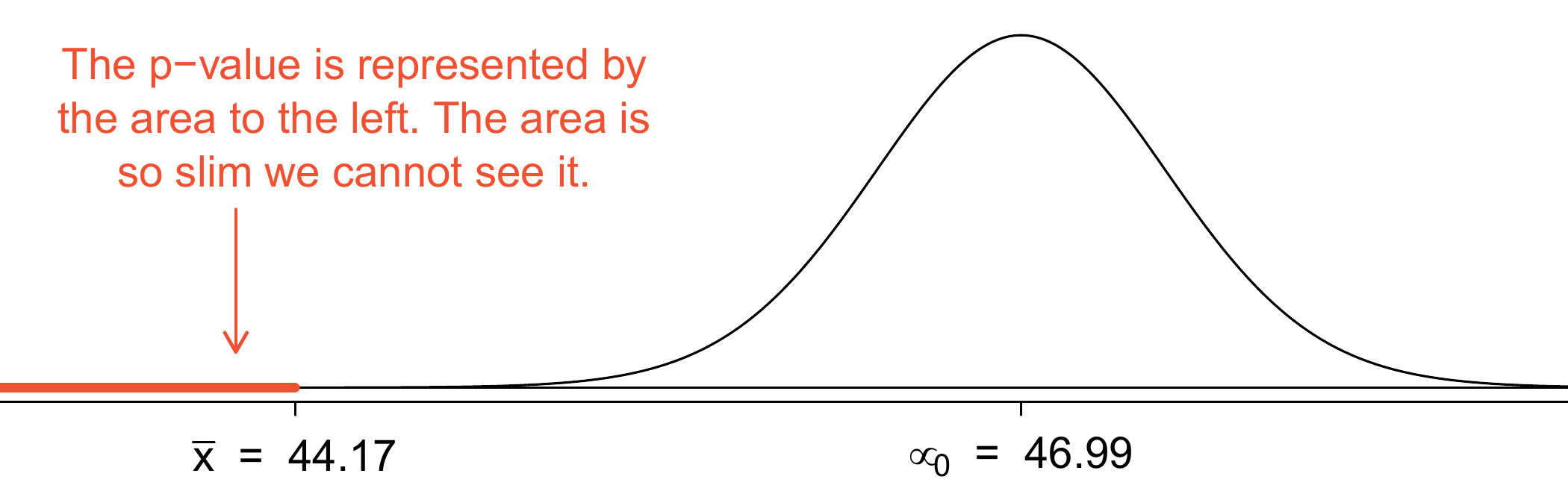
Because the alternative hypothesis says we are looking for a smaller mean, we shade the lower tail. We find this shaded area by using the Z-score and normal probability table: $Z = \frac{44.17 - 46.99}{0.5755} = -4.90$, which has area less than 0.0002. The area is so small we cannot really see it on the picture. This lower tail area corresponds to the p-value.

Because the p-value is so small – specifically, smaller than $\alpha = 0.01$ – this provides sufficiently strong evidence to reject the null hypothesis in favour of the alternative. The data provide statistically significant evidence that the average price on Ebay is lower than Amazon’s asking price.

Definition 9.8 (What’s so special about 0.05?) It’s common to use a threshold of 0.05 to determine whether a result is statistically significant, but why is the most common value 0.05? Maybe the standard significance level should be bigger, or maybe it should be smaller. If you’re a little puzzled, that probably means you’re reading with a critical eye – good job!

9.4 Examining the Central Limit Theorem

The normal model for the sample mean tends to be very good when the sample consists of at least 30 independent observations and the population data are not strongly skewed. The Central Limit Theorem provides the theory that allows us to make this assumption.

Definition 9.9 (Central Limit Theorem, informal definition) The distribution of $\bar{x}$ is approximately normal. The approximation can be poor if the sample size is small, but it improves with larger sample sizes.

The Central Limit Theorem states that when the sample size is small, the normal approximation may not be very good. However, as the sample size becomes large, the normal approximation improves. We will investigate three cases to see roughly when the approximation is reasonable.

We consider three data sets: one from a uniform distribution, one from an exponential distribution, and the other from a log-normal distribution. These distributions are shown in the top panels of Figure 9.11. The uniform distribution is symmetric, the exponential distribution may be considered as having moderate skew since its right tail is relatively short (few outliers), and the log-normal distribution is strongly skewed and will tend to produce more apparent outliers.

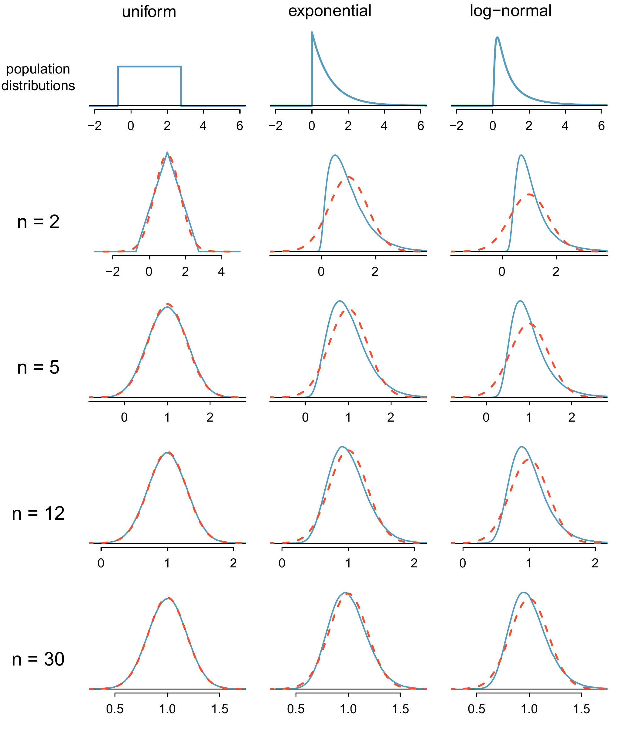
Sampling distributions for the mean at different sample sizes and for three different distributions. The dashed red lines show normal distributions.

Figure 9.11: Sampling distributions for the mean at different sample sizes and for three different distributions. The dashed red lines show normal distributions.

The left panel in the $n=2$ row represents the sampling distribution of $\bar{x}$ if it is the sample mean of two observations from the uniform distribution shown. The dashed line represents the closest approximation of the normal distribution. Similarly, the centre and right panels of the $n=2$ row represent the respective distributions of $\bar{x}$ for data from exponential and log-normal distributions.

Guided Practice9.17
Examine the distributions in each row of Figure 9.11. What do you notice about the normal approximation for each sampling distribution as the sample size becomes larger?¹¹⁰

Example 9.3
Would the normal approximation be good in all applications where the sample size is at least 30?

Not necessarily. For example, the normal approximation for the log-normal example is questionable for a sample size of 30. Generally, the more skewed a population distribution or the more common the frequency of outliers, the larger the sample required to guarantee the distribution of the sample mean is nearly normal.

Remark (With larger $n$, the sampling distribution of $\bar{x}$ becomes more normal). As the sample size increases, the normal model for $\bar{x}$ becomes more reasonable. We can also relax our condition on skew when the sample size is very large.

We discussed in Section 9.1.3 that the sample standard deviation, $s$, could be used as a substitute of the population standard deviation, $\sigma$, when computing the standard error. This estimate tends to be reasonable when $n\geq30$.

Example 9.4
Figure 9.12 shows a histogram of 50 observations. These represent winnings and losses from 50 consecutive days of a professional poker player. Can the normal approximation be applied to the sample mean, 90.69?

We should consider each of the required conditions.

These are referred to as time series data, because the data arrived in a particular sequence. If the player wins on one day, it may influence how she plays the next. To make the assumption of independence we should perform careful checks on such data. While the supporting analysis is not shown, no evidence was found to indicate the observations are not independent.
The sample size is 50, satisfying the sample size condition.
There are two outliers, one very extreme, which suggests the data are very strongly skewed or very distant outliers may be common for this type of data. Outliers can play an important role and affect the distribution of the sample mean and the estimate of the standard error.

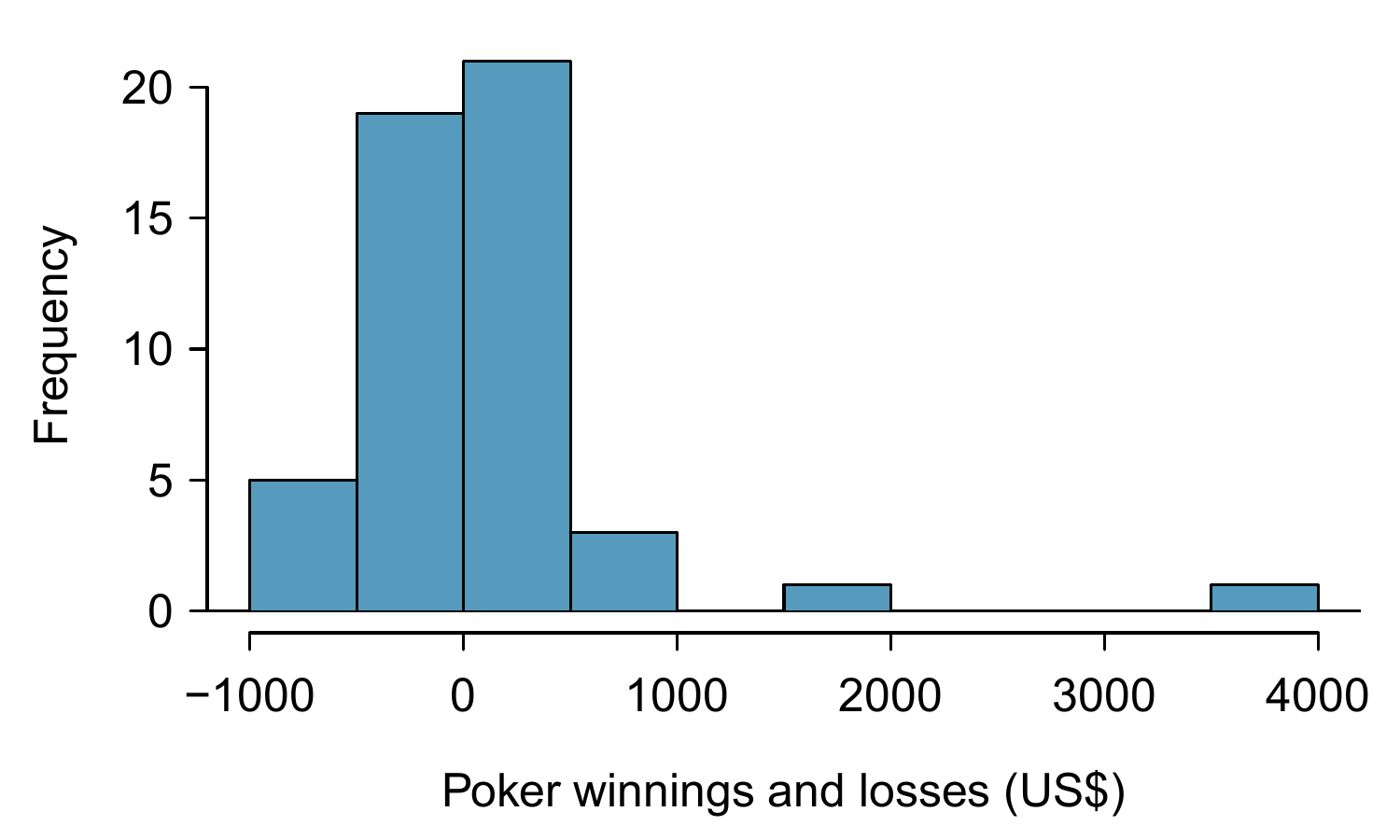
Since we should be sceptical of the independence of observations and the very extreme upper outlier poses a challenge, we should not use the normal model for the sample mean of these 50 observations. If we can obtain a much larger sample, perhaps several hundred observations, then the concerns about skew and outliers would no longer apply.

Sample distribution of poker winnings. These data include some very clear outliers. These are problematic when considering the normality of the sample mean. For example, outliers are often an indicator of very strong skew.

Figure 9.12: Sample distribution of poker winnings. These data include some very clear outliers. These are problematic when considering the normality of the sample mean. For example, outliers are often an indicator of very strong skew.

Remark (Caution: Examine data structure when considering independence). Some data sets are collected in such a way that they have a natural underlying structure between observations, e.g. when observations occur consecutively. Be especially cautious about independence assumptions regarding such data sets.

Remark (Caution: Watch out for strong skew and outliers). Strong skew is often identified by the presence of clear outliers. If a data set has prominent outliers, or such observations are somewhat common for the type of data under study, then it is useful to collect a sample with many more than 30 observations if the normal model will be used for $\bar{x}$.

You won’t be a pro at assessing skew by the end of this book, so just use your best judgement and continue learning. As you develop your statistics skills and encounter tough situations, also consider learning about better ways to analyse skewed data, such as the studentized bootstrap (bootstrap-t), or consult a more experienced statistician.

9.4.1 Statistical significance versus practical significance

When the sample size becomes larger, point estimates become more precise and any real differences in the mean and null value become easier to detect and recognize. Even a very small difference would likely be detected if we took a large enough sample. Sometimes researchers will take such large samples that even the slightest difference is detected. While we still say that difference is statistically significant, it might not be practically significant.

Statistically significant differences are sometimes so minor that they are not practically relevant. This is especially important to research: if we conduct a study, we want to focus on finding a meaningful result. We don’t want to spend lots of money finding results that hold no practical value.

The role of a statistician in conducting a study often includes planning the size of the study. The statistician might first consult experts or scientific literature to learn what would be the smallest meaningful difference from the null value. She also would obtain some reasonable estimate for the standard deviation. With these important pieces of information, she would choose a sufficiently large sample size so that the power for the meaningful difference is perhaps 80% or 90%. While larger sample sizes may still be used, she might advise against using them in some cases, especially in sensitive areas of research.

www.cdc.gov/healthyyouth/data/yrbs/data.htm↩︎
(a) Consider two random samples: one of size 10 and one of size 1000. Individual observations in the small sample are highly influential on the estimate while in larger samples these individual observations would more often average each other out. The larger sample would tend to provide a more accurate estimate. (b) If we think an estimate is better, we probably mean it typically has less error. Based on (a), our intuition suggests that a larger sample size corresponds to a smaller standard error.↩︎
(a) Use Equation (9.1) with the sample standard deviation to compute the standard error: $SE_{\bar{y}} = 0.088 / \sqrt{100} = 0.0088$ meters. (b) It would not be surprising. Our sample is about 1 standard error from 1.69m. In other words, 1.69m does not seem to be implausible given that our sample was relatively close to it. (We use the standard error to identify what is close.)↩︎
(a) Extra observations are usually helpful in understanding the population, so a point estimate with 400 observations seems more trustworthy. (b) The standard error when the sample size is 100 is given by $SE_{100} = 10/\sqrt{100} = 1$. For 400: $SE_{400} = 10/\sqrt{400} = 0.5$. The larger sample has a smaller standard error. (c) The standard error of the sample with 400 observations is lower than that of the sample with 100 observations. The standard error describes the typical error, and since it is lower for the larger sample, this mathematically shows the estimate from the larger sample tends to be better – though it does not guarantee that every large sample will provide a better estimate than a particular small sample.↩︎
If we want to be more certain we will capture the fish, we might use a wider net. Likewise, we use a wider confidence interval if we want to be more certain that we capture the parameter.↩︎
Just as some observations occur more than 2 standard deviations from the mean, some point estimates will be more than 2 standard errors from the parameter. A confidence interval only provides a plausible range of values for a parameter. While we might say other values are implausible based on the data, this does not mean they are impossible.↩︎
https://www.theloquitur.com/pollshowscollegestudentsgetleastamountofsleep/↩︎
While we could answer this question by examining the entire YRBSS data set from 2013 (yrbss), we only consider the sample data (yrbss_samp), which is more realistic since we rarely have access to population data.↩︎
The jury considers whether the evidence is so convincing (strong) that there is no reasonable doubt regarding the person’s guilt; in such a case, the jury rejects innocence (the null hypothesis) and concludes the defendant is guilty (alternative hypothesis).↩︎
If the court makes a Type 1 Error, this means the defendant is innocent ($H_0$ true) but wrongly convicted. A Type 2 Error means the court failed to reject $H_0$ (i.e. failed to convict the person) when she was in fact guilty ($H_A$ true).↩︎
To lower the Type~1 Error rate, we might raise our standard for conviction from “beyond a reasonable doubt” to “beyond a conceivable doubt” so fewer people would be wrongly convicted. However, this would also make it more difficult to convict the people who are actually guilty, so we would make more Type 2 Errors.↩︎
To lower the Type 2 Error rate, we want to convict more guilty people. We could lower the standards for conviction from “beyond a reasonable doubt” to “beyond a little doubt.” Lowering the bar for guilt will also result in more wrongful convictions, raising the Type 1 Error rate.↩︎
A sceptic would have no reason to believe that sleep patterns at this school are different to the sleep patterns at another school.↩︎
This is entirely based on the interests of the researchers. Had they been only interested in the opposite case – showing that their students were actually averaging fewer than seven hours of sleep but not interested in showing more than 7 hours – then our setup would have set the alternative as $\mu < 7$.↩︎
The standard error can be estimated from the sample standard deviation and the sample size: $SE_{\bar{x}} = \frac{s_x}{\sqrt{n}} = \frac{1.75}{\sqrt{110}} = 0.17$.↩︎
About 5% of the time. If the null hypothesis is true, then the data only has a 5% chance of being in the 5% of data most favourable to $H_A$.↩︎
We reject the null hypothesis whenever $p$-$value < \alpha$. Thus, we would still reject the null hypothesis if $\alpha = 0.01$ but not if the significance level had been $\alpha = 0.001$.↩︎
The sceptic would say the average is the same on Ebay, and we are interested in showing the average price is lower.__[$H_0$:] The average auction price on Ebay is equal to (or more than) the price on Amazon. We write only the equality in the statistical notation: $\mu_{ebay} = 46.99$. [$H_A$:]__ The average price on Ebay is less than the price on Amazon, $\mu_{ebay} < 46.99$.↩︎
These data were collected by OpenIntro staff.↩︎
(1) The independence condition is unclear. We will make the assumption that the observations are independent, which we should report with any final results. (2) The sample size is sufficiently large: $n =52 \geq 30$. (3) The data distribution is not strongly skewed; it is approximately symmetric.↩︎
The normal approximation becomes better as larger samples are used.↩︎

	Conclusion:do no reject \(H_0\)	Conclusion: reject \(H_0\) in favour of \(H_A\)
\(H_0\) true	okay	Type 1 error
	\((1-\alpha)\)	\((\alpha)\)
\(H_A\) true	Type 2 error	okay
	\((\beta)\)	\((1-\beta)\)

Variable	Description
\(\texttt{age}\)	Age of the student.
\(\texttt{gender}\)	Sex of the student.
\(\texttt{grade}\)	Grade in high school
\(\texttt{height}\)	Height, in meters. There are 3.28 feet in a meter.
\(\texttt{weight}\)	Weight, in kilograms (2.2 pounds per kilogram).
\(\texttt{helmet}\)	Frequency that the student wore a helmet while biking in the last 12~months.
\(\texttt{active}\)	Number of days physically active for 60+ minutes in the last 7 days.
\(\texttt{lifting}\)	Number of days of strength training (e.g. lifting weights) in the last 7 days.