Chapter 6 Graphical Parameters
One of the beneficial things about using R is that it allows you flexibility when creating figures. With R you can easily customise plots using a seemingly endless array of functions and parameters. This guide will cover how to specify colour, symbols and line types, and how to save plots. Many other graphical parameters and functions are covered within other guides for this unit.
6.1 Defining Colours
Colours can be defined for a number of different attributes in R (e.g. points, lines and text). The standard parameter for most functions with colour capabilities is col, and this can be defined by a number or name, or a vector of either of these using the function concatenate c(). When defining a vector, colours are separated by a comma and enclosed in (parentheses). If colours are defined as names, they must be each enclosed in “double quotes.” The default colour is almost always black, and the standard colour numbers run from 1 to 8 (see Figure 6.1). Outside of these colours there are hundreds more available - more easily by name - which can be found by executing this command in your R console: colours(). You can also find colour charts online by searching “R colours.” The following are just a few examples of how col can be defined in R:
# specify colour by number
  col= 1,          # black
  col= c(1,2,3),   # vector of colours 1,2,3
  col= c(1:3),     # range of colours 1 to 3 - same as above
# specify colour by name
  col= "grey",
col= c("grey10","grey30","grey80"), par(mfrow=c(1,1),mar=c(3,0,2,0))
x <- rep(1:8)
y <- rep(1, times = 8)
plot(x,y, col= 1:8, pch= 15, cex= 3, ylim= c(0,2), yaxt= "n",
main= "Colour Numbers in R: 'col = 1 to 8'")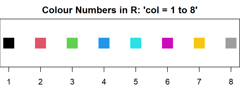
Figure 6.1: Plot showing standard colour numbers (1 to 8) in R.
6.2 Defining Symbols (Points)
Symbols can be defined to customize plot points, or differentiate points for different groups of a categorical variable (e.g. species or treatments). The parameter for point type is pch (Point CHange) and this can be defined as a number relating to one of the default symbols (1 to 25 - see Figure 6.2) or as a keyboard character or character string (i.e. group name). If points are defined as characters they must be enclosed in “double quotes.” Points can also be given as a vector using the function c(). The size of your points can be changed with parameter cex by providing the proportion to increase or decrease from the default size. Lastly, while the colour can be changed for all points, default points 21 to 25 can have both the fill and outline defined using parameters bg and col. Here are a few examples:
# default point types by number
  pch= 1,              # circle outline
  pch= c(1,2,3),       # vector of points 1,2,3
  pch= c(1:3),         # range of points 1 to 3 - same as above
# setting points as characters
  pch= "A",
  pch= c("N","S","E","W"),
# point size (cex)
  pch= 1, cex= 0.5,         # circle outline, 50% the default size
  pch= c(1,2,3), cex= 1.2,  # points 1,2,3, all 20% larger than default
# add colour (col,bg)
  pch= 1, col= 4,           # blue circle outline
  pch= 21, col= 3, bg= 1,   # filled green circle with black outline
# combine parameters
# points 1,2,5 all 20% larger, and using colours 2 to 4
  pch= c(1,2,5), cex= 1.2, col= c(2:4),

# the most common situation for changing the points is for a scatter plot
# for example:
with(my.data,plot(Y.values ~ X.values, cex= 2, col=1, bg=8))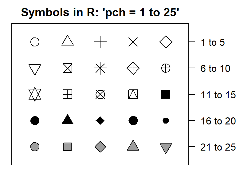
Figure 6.2: Plot showing available symbols by number in R. Note symbols 21 to 25 have background/fill defined as grey (bg = 8) and outline defined as black (col = 1)
6.3 Defining Line Types
Line types are defined in R by the parameter lty (Line TYpe) and there are 6 options to choose from (see Figure 6.3). You can also set the width of your line with parameter lwd (Line WiDth), with larger numbers giving thicker lines.
# line type
  lty= 1,              # solid line
  lty= c(1,5,3),       # list of lines 1,5,3
  lty= c(1:6),         # range of points 1 to 3 - same as above
# line width
  lty= 1, lwd= 0.5,         # solid lines, 50% default size
  lty= c(1,2,3), lwd= 1.2,  # lines 1,2,3, all 20% larger
# add colour
  lty= 1, col= 4,           # blue solid line
  lty= c(1,5), col= c(3,4), # green solid and blue dashed lines
# combine all parameters
# lines 1,2,3, all red, and using line widths 2 to 4
  lty= c(1,2,3), col= 2, lwd= c(2:4),
#  the most common situation for controlling the line type is adding
#  the trend line to a scatter plot.  For example:
abline(lm.1, col = 2, lty= 2, lwd= 2)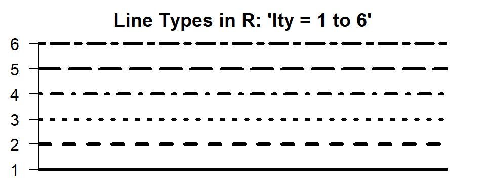
Figure 6.3: Plot showing available line types in R (1 to 6).
6.4 Saving Plots
The best and most efficient way to get high quality graphics from R is to save them from the command line. There are three steps to save a plot:
- specify the file details - this starts a device which creates an empty file and waits for you to provide the contents (i.e. a plot). Here you can specify the following parameters:
- file type: this determines the command you use, e.g.
png(),jpeg(),tiff(),bmp() - file name: choose something intuitive; file name and extension must be included and enclosed in “double quotes” (e.g.
"My_file_name.png") - directory: by default the plot will be saved to your working directory; if you prefer another, specify this with the file name using forward slashes between directories (Windows operating systems use backward slashes to indicate paths and R will not recognize this!)
- figure size: specify this with optional parameters
width,heightandunits(‘mm,’ ‘cm,’ ‘in,’ default= ‘pixels’); since figures can easily be enlarged and compressed, e.g. when pasted into a MS Word document, this determines the plot size relative to its contents, axes and title. E.g. if your boxes seem squished in your box plot at a height of 70 mm, increase it to 100 mm. This will NOT change the actual axis value. - resolution: the default for parameter
resis 72 pixels per inch (ppi), a good quality photograph generally requires 300. Set this if you require high quality figures (i.e. for a report/assignment), recognizing resolution is relevant for the size the plot is saved at.
- file type: this determines the command you use, e.g.
- create your plot as you would normally
- close the device - this is the step that actually SAVES your plot
Here is an example of what this looks like in R:
#1. Create an empty file in your working directory with your
#   specified parameters
png("Figure1.png", width = 100, height = 100, units = 'mm', res = 300)

#2. Create your plot
with(PlantGrowth,hist(weight,
      xlim= c(3,7),                       # set the x-axis range
      ylim= c(0,10),                      # set the y-axis range
      col= "lightgray",                   # fill the columns
      border= "black",                    # column border
      main= "Histogram of Plant Weights", # figure title
      xlab= "Dried weight (g)",           # x-axis label
      ylab= "Frequency"))                 # y-axis label

#3. Save your plot by turning device off
dev.off()
For information on which file type to choose, see the R help file: BMP, JPEG, PNG and TIFF graphics devices. In general, tiff files are larger but better quality figures. Also note that some `viewer’ applications do not support all file types (tiff are widely accepted). If when trying to view your saved plot you receive an error, try to open it with another application.