Chapter 8 Distributions

8.1 Normal Distribution

Among all the distributions we see in practice, one is overwhelmingly the most common. The symmetric, unimodal, bell curve is ubiquitous throughout statistics. Indeed it is so common, that people often know it as the normal curve or normal distribution⁵⁰, shown in Figure 8.1. Many variables observed in nature closely follow the normal distribution.

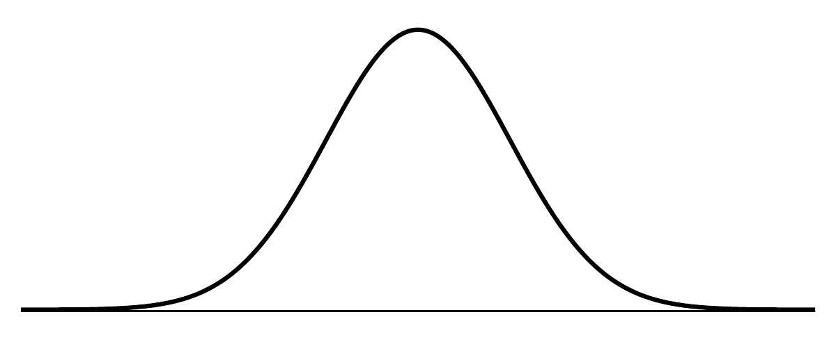
Figure 8.1: A normal curve.

Definition 8.1 (Normal distribution facts) Many variables are nearly normal, but none are exactly normal. Thus the normal distribution, while not perfect for any single problem, is very useful for a variety of problems. We will use it in data exploration and to solve important problems in statistics.

8.1.1 Normal distribution model

The normal distribution model always describes a symmetric, unimodal, bell-shaped curve. However, these curves can look different depending on the details of the model. Specifically, the normal distribution model can be adjusted using two parameters: mean and standard deviation. As you can probably guess, changing the mean shifts the bell curve to the left or right, while changing the standard deviation stretches or constricts the curve. Figure 8.2 shows the normal distribution with mean \(0\) and standard deviation \(1\) in the left panel and the normal distributions with mean \(19\) and standard deviation \(4\) in the right panel. Figure 8.3 shows these distributions on the same axis.

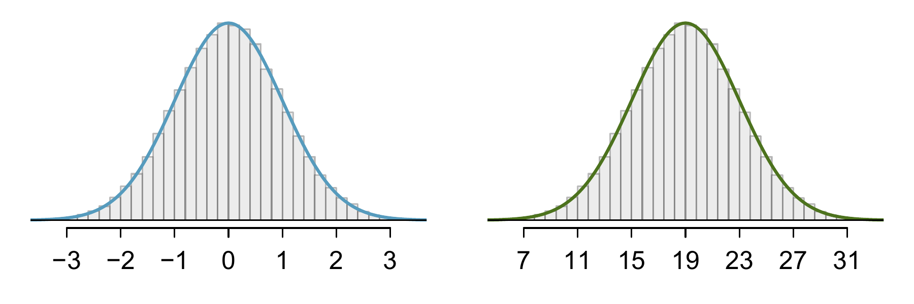
Figure 8.2: Both curves represent the normal distribution, however, they differ in their centre and spread. The normal distribution with mean 0 and standard deviation 1 is called the standard normal distribution.

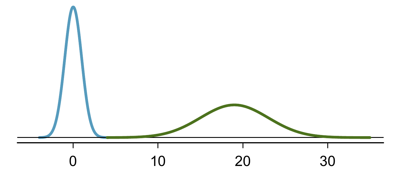
Figure 8.3: The normal models shown in Figure 8.2 but plotted together and on the same scale.“,fig.scap=”Illustration of two normal distributions, on same scale.

If a normal distribution has mean \(\mu\) and standard deviation \(\sigma\), we may write the distribution as \(N(\mu, \sigma)\). The two distributions in Figure 8.3 can be written as \[ \begin{aligned} N(\mu=0,\sigma=1)\quad\text{and}\quad N(\mu=19,\sigma=4) \end{aligned} \] Because the mean and standard deviation describe a normal distribution exactly, they are called the distribution’s parameter.

Guided Practice8.1 Write down the short-hand for a normal distribution with⁵¹

1. mean5 and standard deviation 3,
2. mean-100 and standard deviation 10, and
3. mean 2 and standard deviation 9.

8.1.2 Standardizing with \(Z\)-scores

Example 8.1 Table 8.1 shows the mean and standard deviation for total scores on two aptitude tests for entrance to US universities, the SAT and ACT. The distribution of SAT and ACT scores are both nearly normal. Suppose Ann scored 1800 on her SAT and Tom scored 24 on his ACT. Who performed better?
We use the standard deviation as a guide. Ann is 1 standard deviation above average on the SAT: \(1500 + 300=1800\). Tom is 0.6 standard deviations above the mean on the ACT: \(21+0.6\times 5=24\). In Figure 8.4, we can see that Ann tends to do better with respect to everyone else than Tom did, so her score was better.

Table 8.1: Summary statistics.

Summary metric	SAT	ACT
Mean	1500	21
SD	300	5

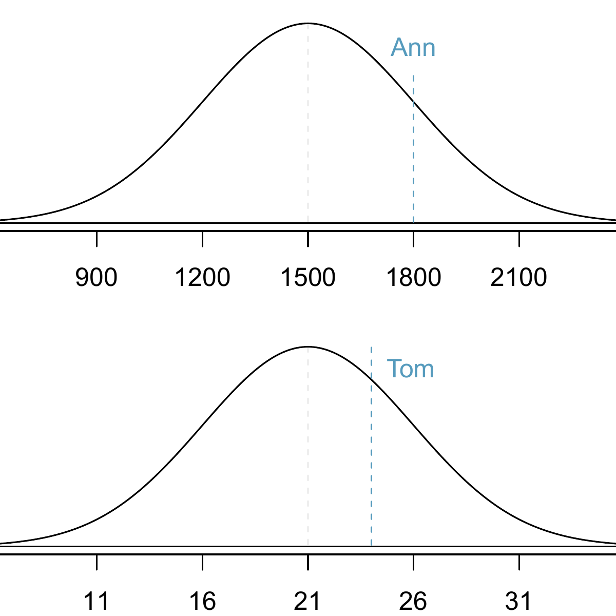
Figure 8.4: Ann’s and Tom’s scores shown with the distributions of SAT and ACT scores.

Example 8.1 used a standardization technique called a \(Z\)-score, a method most commonly employed for nearly normal observations but that may be used with any distribution. The \(Z\)-score of an observation is defined as the number of standard deviations it falls above or below the mean. If the observation is one standard deviation above the mean, its \(Z\)-score is 1. If it is 1.5 standard deviations the mean, then its \(Z\)-score is -1.5. If \(x\) is an observation from a distribution \(N(\mu, \sigma)\), we define the \(Z\)-score mathematically as

\[ Z = \frac{x-\mu}{\sigma} \] Using \(\mu_{SAT}=1500\), \(\sigma_{SAT}=300\), and \(x_{Ann}=1800\), we find Ann’s \(Z\)-score: \[ Z_{Ann} = \frac{x_{Ann} - \mu_{SAT}}{\sigma_{SAT}} = \frac{1800-1500}{300} = 1 \]

Definition 8.2 (The \(Z\)-score) The \(Z\)-score of an observation is the number of standard deviations it falls above or below the mean. We compute the \(Z\)-score for an observation \(x\) that follows a distribution with mean \(\mu\) and standard deviation \(\sigma\) using \[ Z = \frac{x-\mu}{\sigma} \]

Guided Practice8.2 Use Tom’s ACT score, 24, along with the ACT mean and standard deviation to compute his \(Z\)-score.⁵²

Observations above the mean always have positive \(Z\)-scores while those below the mean have negative \(Z\)-scores. If an observation is equal to the mean (e.g. SAT score of 1500), then the \(Z\)-score is \(0\).

Guided Practice8.3 Let \(X\) represent a random variable from \(N(\mu=3, \sigma=2)\), and suppose we observe \(x=5.19\).

1. Find the \(Z\)-score of \(x\).
   
2. Use the \(Z\)-score to determine how many standard deviations above or below the mean \(x\) falls.⁵³

Guided Practice8.4 Head lengths of brushtail possums follow a nearly normal distribution with mean 92.6 mm and standard deviation 3.6 mm. Compute the \(Z\)-scores for possums with head lengths of 95.4 mm and 85.8 mm.⁵⁴

We can use \(Z\)-scores to roughly identify which observations are more unusual than others. One observation \(x_1\) is said to be more unusual than another observation \(x_2\) if the absolute value of its \(Z\)-score is larger than the absolute value of the other observation’s \(Z\)-score: \(|Z_1| > |Z_2|\). This technique is especially insightful when a distribution is symmetric.

Guided Practice8.5 Which of the observations in Guided Practice 8.4 is more unusual?⁵⁵

We can use the normal model to find percentiles. A normal probability table, which lists \(Z\)-scores and corresponding percentiles used to be used to identify a percentile based on the \(Z\)-score (and vice versa). Looking up statistical tables is no longer needed as finding these values in R and other software is very simple.

# calculate the probability P(Z<0.43) - i.e. what is the probability of standard
# normal variable taking a value less than 0.43?
pnorm(q = 0.43, mean = 0, sd = 1)
#> [1] 0.666
# calculate the $Z$-score satisfying P(Z<z)=0.80 - i.e. what value is at the 80th
# percentile of a standard normal distribution?
qnorm(p = 0.8, mean = 0, sd = 1)
#> [1] 0.842
# to see more options, type '?rnorm'

Guided Practice8.6 Determine the proportion of SAT test takers who scored better than Ann on the SAT.⁵⁶

8.1.3 Normal probability examples

Cumulative SAT scores are approximated well by a normal model, \(N(\mu=1500, \sigma=300)\).

Example 8.2 Shannon is a randomly selected SAT taker, and nothing is known about Shannon’s SAT aptitude. What is the probability Shannon scores at least 1630 on her SATs?

First, always draw and label a picture of the normal distribution. (Drawings need not be exact to be useful.) We are interested in the chance she scores above 1630, so we shade this upper tail:

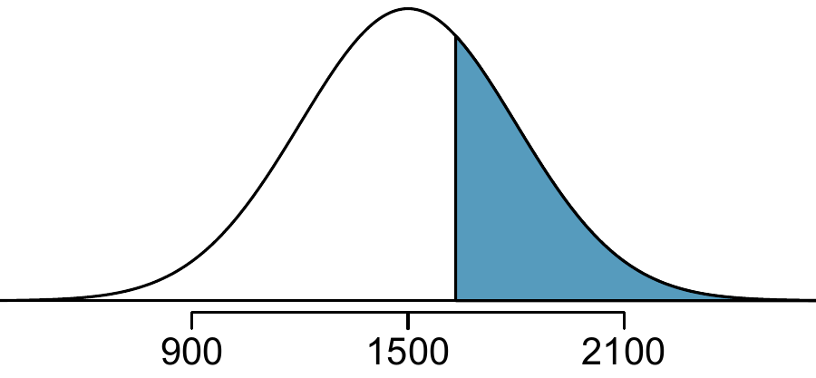
The picture shows the mean and the values at 2 standard deviations above and below the mean. The simplest way to find the shaded area under the curve makes use of the \(Z\)-score of the cutoff value. With \(\mu=1500\), \(\sigma=300\), and the cutoff value \(x=1630\), the \(Z\)-score is computed as \[ Z = \frac{x - \mu}{\sigma} = \frac{1630 - 1500}{300} = \frac{130}{300} = 0.43 \] We look up the percentile of \(Z=0.43\) in the normal probability table or using statistical software, which yields 0.6664. However, the percentile describes those who had a \(Z\)-score than 0.43. To find the area \(Z=0.43\), we compute one minus the area of the lower tail:

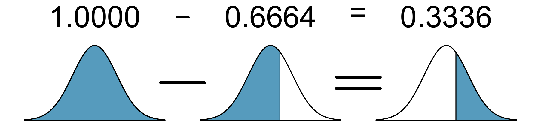The probability Shannon scores at least 1630 on the SAT is 0.3336.

Remark (always draw a picture first, and find the \(Z\)-score second). For any normal probability situation, draw and label the normal curve and shade the area of interest first. The picture will provide an estimate of the probability.
After drawing a figure to represent the situation, identify the \(Z\)-score for the observation of interest.

Guided Practice8.7 If the probability of Shannon scoring at least 1630 is 0.3336, then what is the probability she scores less than 1630? Draw the normal curve representing this exercise, shading the lower region instead of the upper one.⁵⁷

Example 8.3 Edward earned a 1400 on his SAT. What is his percentile?

First, a picture is needed. Edward’s percentile is the proportion of people who do not get as high as a 1400. These are the scores to the left of 1400.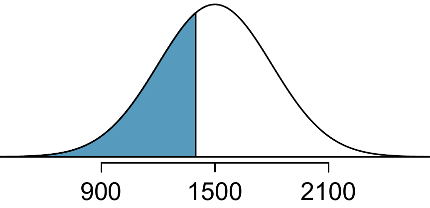 Identifying the mean \(\mu=1500\), the standard deviation \(\sigma=300\), and the cutoff for the tail area \(x=1400\) makes it easy to compute the \(Z\)-score: \[ Z = \frac{x - \mu}{\sigma} = \frac{1400 - 1500}{300} = -0.33 \] Using the normal probability table, identify the row of \(-0.3\) and column of \(0.03\), which corresponds to the probability \(0.3707\). Edward is at the \(37^{th}\) percentile.

Guided Practice8.8 Use the results of Example 8.3 to compute the proportion of SAT takers who did better than Edward. Also draw a new picture.⁵⁸

Remark (areas to the right). The normal probability table in most books gives the area to the left. If you would like the area to the right, first find the area to the left and then subtract this amount from~one.

Guided Practice8.9 Stuart earned an SAT score of 2100. Draw a picture for each part.

1. What is his percentile?
   
2. What percent of SAT takers did better than Stuart?⁵⁹

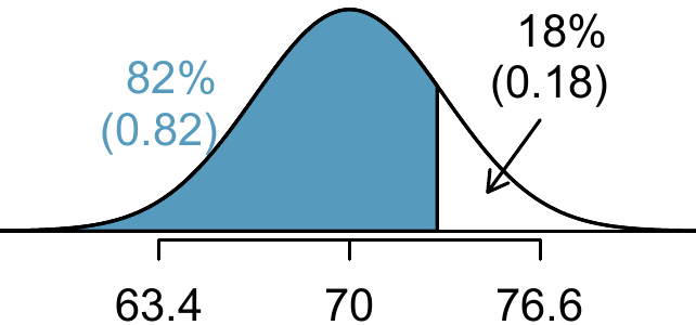
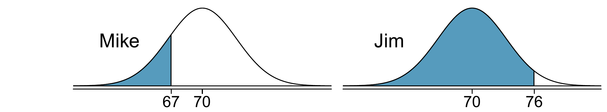
Based on a sample of 100 men,⁶⁰ the heights of male adults between the ages 20 and 62 in the US is nearly normal with mean 70.0’’ and standard deviation 3.3’’.

Guided Practice8.10 Mike is 5’7’’ and Jim is 6’4’’.

1. What is Mike’s height percentile?
   
2. What is Jim’s height percentile?

Also draw one picture for each part.⁶¹

The last several problems have focused on finding the probability or percentile for a particular observation. What if you would like to know the observation corresponding to a particular percentile?

Example 8.4 Erik’s height is at the \(40^{th}\) percentile. How tall is he?

As always, first draw the picture.

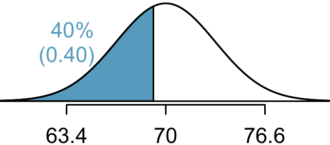
In this case, the lower tail probability is known (0.40), which can be shaded on the diagram. We want to find the observation that corresponds to this value. As a first step in this direction, we determine the \(Z\)-score associated with the \(40^{th}\) percentile.

Because the percentile is below 50%, we know \(Z\) will be negative. Looking in the negative part of the normal probability table, we search for the probability inside the table closest to 0.4000. We find that 0.4000 falls in row \(-0.2\) and between columns \(0.05\) and \(0.06\). Since it falls closer to \(0.05\), we take this one: \(Z=-0.25\).

Knowing \(Z_{Erik}=-0.25\) and the population parameters \(\mu=70\) and \(\sigma=3.3\) inches, the \(Z\)-score formula can be set up to determine Erik’s unknown height, labelled \(x_{Erik}\): \[ -0.25 = Z_{Erik} = \frac{x_{Erik} - \mu}{\sigma} = \frac{x_{Erik} - 70}{3.3} \] Solving for \(x_{Erik}\) yields the height 69.18 inches. That is, Erik is about 5’9’’ (this is notation for 5-feet, 9-inches).

Example 8.5 What is the adult male height at the \(82^{nd}\) percentile?

Again, we draw the figure first.

Next, we want to find the \(Z\)-score at the \(82^{nd}\) percentile, which will be a positive value. Looking in the Z-table, we find \(Z\) falls in row \(0.9\) and the nearest column is \(0.02\), i.e. \(Z=0.92\). Finally, the height \(x\) is found using the \(Z\)-score formula with the known mean \(\mu\), standard deviation \(\sigma\), and \(Z\)-score \(Z=0.92\): \[ 0.92 = Z = \frac{x-\mu}{\sigma} = \frac{x - 70}{3.3} \] This yields 73.04 inches or about 6’1’’ as the height at the \(82^{nd}\) percentile.

Guided Practice8.11  
(a) What is the \(95^{th}\) percentile for SAT scores?
(b) What is the \(97.5^{th}\) percentile of the male heights? As always with normal probability problems, first draw a picture.⁶²

Guided Practice8.12  
(a) What is the probability that a randomly selected male adult is at least 6’2’’ (74 inches)?
(b) What is the probability that a male adult is shorter than 5’9’’ (69 inches)?⁶³

Example 8.6 What is the probability that a random adult male is between 5’9’’ and 6’2’’?

These heights correspond to 69 inches and 74 inches. First, draw the figure. The area of interest is no longer an upper or lower tail.

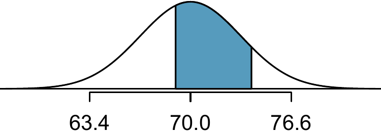
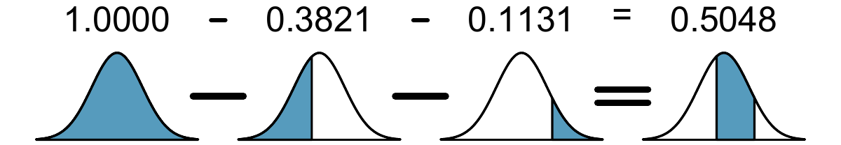
The total area under the curve is 1. If we find the area of the two tails that are not shaded (from Guided Practice 8.12, these areas are \(0.3821\) and \(0.1131\)), then we can find the middle area:

That is, the probability of being between 5’9’’ and 6’2’’ is 0.5048.

Guided Practice8.13 What percent of SAT takers get between 1500 and 2000?⁶⁴

Guided Practice8.14 What percent of adult males are between 5’5’’ and 5’7’’?⁶⁵

8.1.4 68-95-99.7 rule

Here, we present a useful rule of thumb for the probability of falling within 1, 2, and 3 standard deviations of the mean in the normal distribution. This will be useful in a wide range of practical settings, especially when trying to make a quick estimate without a calculator or Z-table.

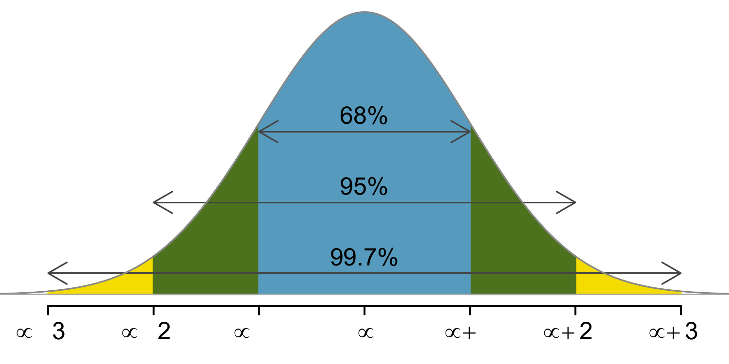
Figure 8.5: Probabilities for falling within 1, 2 and 3 standard deviations of the mean in a normal distribution.

Guided Practice8.15 Use the Z-table to confirm that about 68%, 95%, and 99.7% of observations fall within 1, 2, and 3, standard deviations of the mean in the normal distribution, respectively. For instance, first find the area that falls between \(Z=-1\) and \(Z=1\), which should have an area of about 0.68. Similarly there should be an area of about 0.95 between \(Z=-2\) and \(Z=2\).⁶⁶

It is possible for a normal random variable to fall 4,~5, or~even more standard deviations from the mean. However, these occurrences are very rare if the data are nearly normal. The probability of being further than 4 standard deviations from the mean is about 1-in-15,000. For 5 and 6 standard deviations, it is about 1-in-2 million and 1-in-500 million, respectively.

Guided Practice8.16 SAT scores closely follow the normal model with mean \(\mu = 1500\) and standard deviation \(\sigma = 300\).

1. About what percent of test takers score 900 to 2100?
   
2. What percent score between 1500 and 2100?⁶⁷

8.2 Evaluating the Normal Approximation

Many processes can be well approximated by the normal distribution. We have already seen two good examples: SAT scores and the heights of US adult males. While using a normal model can be extremely convenient and helpful, it is important to remember normality is always an approximation. Testing the appropriateness of the normal assumption is a key step in many data analyses.

Example 8.4 suggests the distribution of heights of US males is well approximated by the normal model. We are interested in proceeding under the assumption that the data are normally distributed, but first we must check to see if this is reasonable.

There are two visual methods for checking the assumption of normality, which can be implemented and interpreted quickly. The first is a simple histogram with the best fitting normal curve overlaid on the plot, as shown in the left panel of Figure 8.6. The sample mean \(\bar{x}\) and standard deviation \(s\) are used as the parameters of the best fitting normal curve. The closer this curve fits the histogram, the more reasonable the normal model assumption. Another more common method is examining a normal probability plot,⁶⁸ shown in the right panel of Figure 8.6. The closer the points are to a perfect straight line, the more confident we can be that the data follow the normal model.

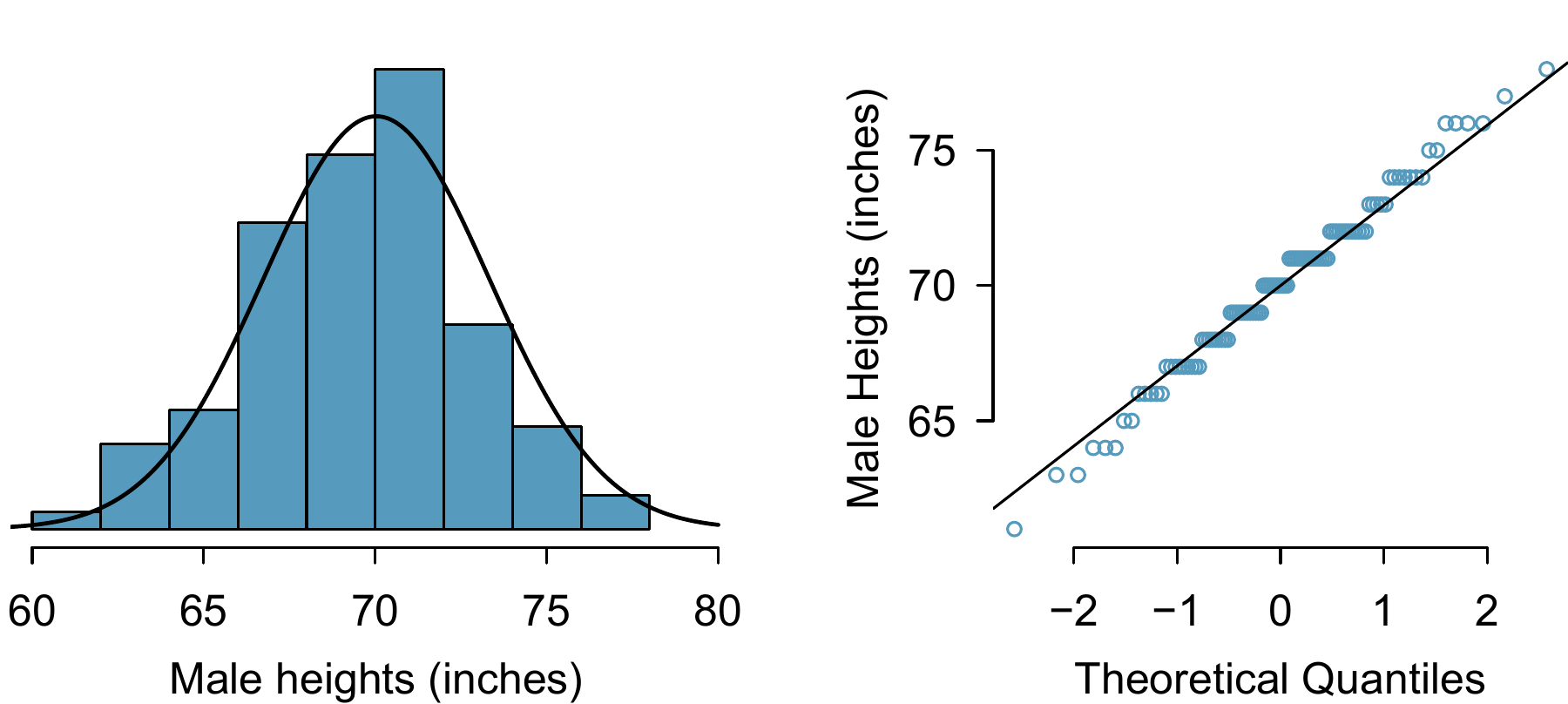
Figure 8.6: A sample of 100 male heights. The observations are rounded to the nearest whole inch, explaining why the points appear to jump in increments in the normal probability plot.

Example 8.7 Three data sets of 40, 100, and 400 samples were simulated from a normal distribution, and the histograms and normal probability plots of the data sets are shown in Figure 8.7. These will provide a benchmark for what to look for in plots of real data.

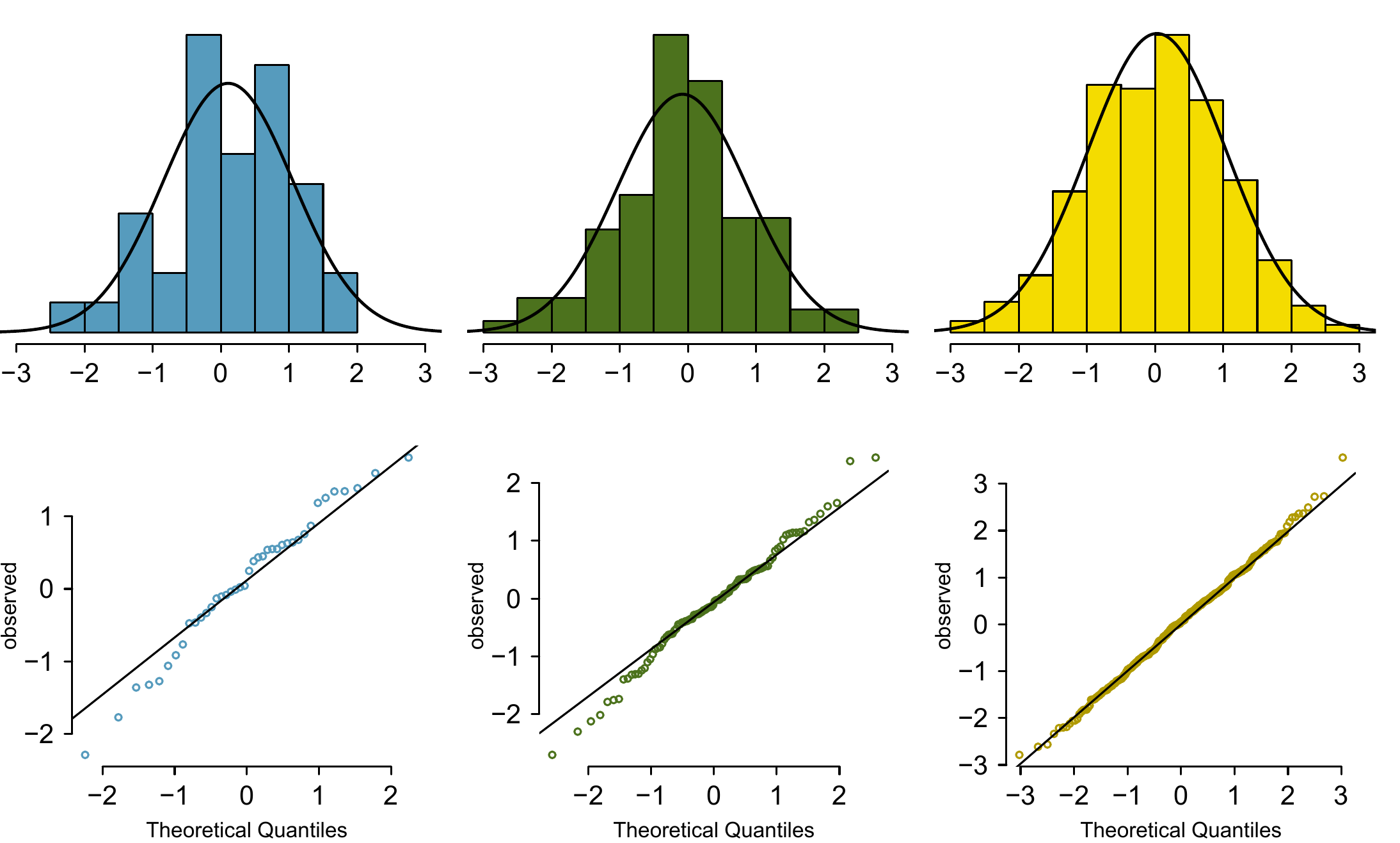
Figure 8.7: Histograms and normal probability plots for three simulated normal data sets; \(n=40\) (left), \(n=100\) (middle), \(n=400\) (right).

The left panels show the histogram (top) and normal probability plot (bottom) for the simulated data set with 40 observations. The data set is too small to really see clear structure in the histogram. The normal probability plot also reflects this, where there are some deviations from the line. We should expect deviations of this amount for such a small data set.

The middle panels show diagnostic plots for the data set with 100 simulated observations. The histogram shows more normality and the normal probability plot shows a better fit. While there are a few observations that deviate noticeably from the line, they are not particularly extreme.

The data set with 400 observations has a histogram that greatly resembles the normal distribution, while the normal probability plot is nearly a perfect straight line. Again in the normal probability plot there is one observation (the largest) that deviates slightly from the line. If that observation had deviated 3 times further from the line, it would be of greater importance in a real data set. Apparent outliers can occur in normally distributed data but they are rare.

Notice the histograms look more normal as the sample size increases, and the normal probability plot becomes straighter and more stable.

Example 8.8 Are NBA player heights normally distributed? Consider all 435 NBA players from the 2008-9 season presented in Figure 8.8.⁶⁹ We first create a histogram and normal probability plot of the NBA player heights. The histogram in the left panel is slightly left skewed, which contrasts with the symmetric normal distribution. The points in the normal probability plot do not appear to closely follow a straight line but show what appears to be a “wave.” We can compare these characteristics to the sample of 400 normally distributed observations in Example 8.7 and see that they represent much stronger deviations from the normal model. NBA player heights do not appear to come from a normal distribution.

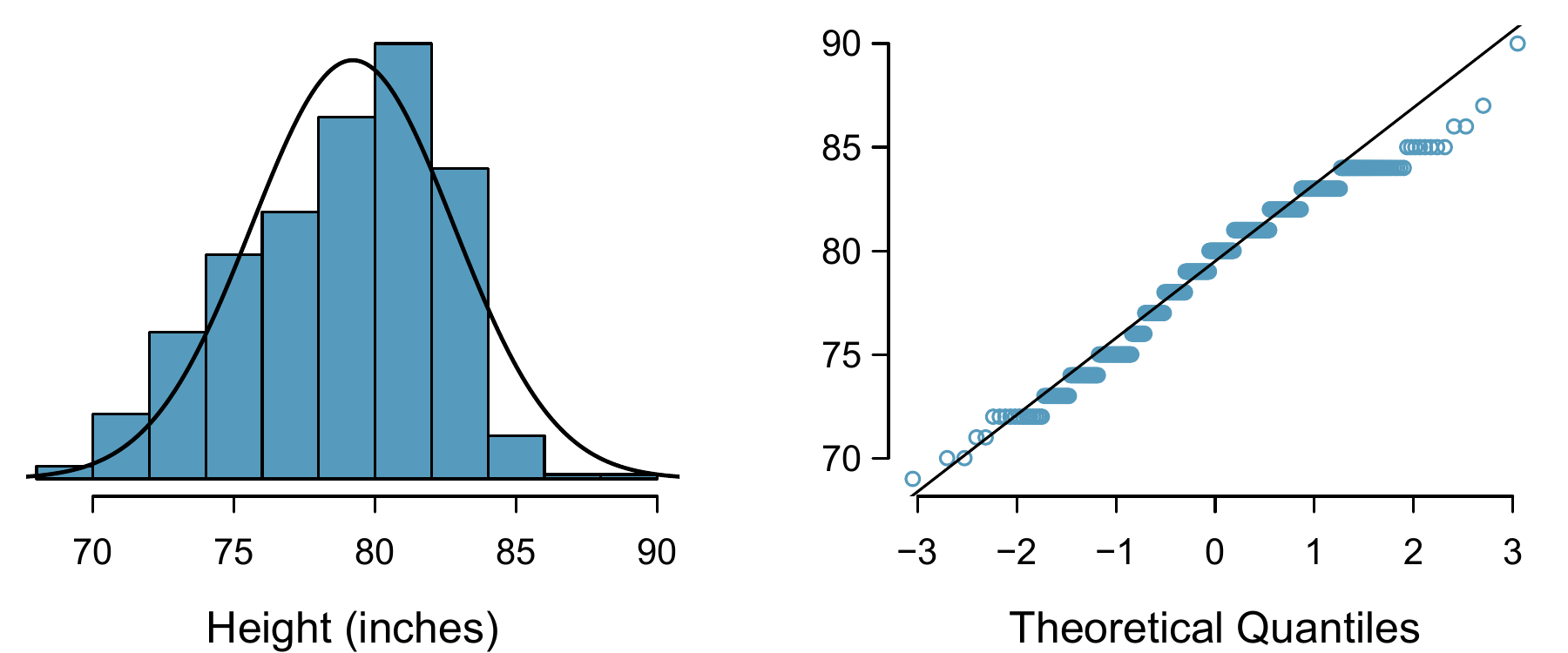
Figure 8.8: Histogram and normal probability plot for the NBA heights from the 2008-9 season.

Example 8.9 Can we approximate poker winnings by a normal distribution? We consider the poker winnings of an individual over 50 days. A histogram and normal probability plot of these data are shown in Figure 8.9. The data are very strongly right skewed in the histogram, which corresponds to the very strong deviations on the upper right component of the normal probability plot. If we compare these results to the sample of 40 normal observations in Example 8.7, it is apparent that these data show very strong deviations from the normal model.

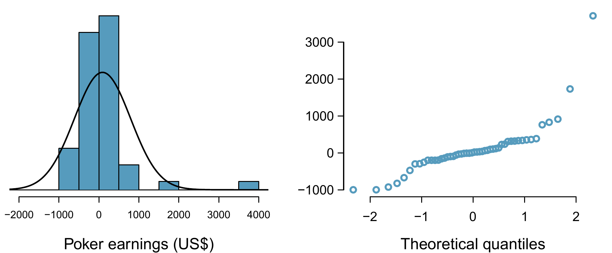
Figure 8.9: A histogram of poker data with normal plot fit and normal probability plot.

Guided Practice8.17 Determine which data sets represented in Figure 8.10 plausibly come from a nearly normal distribution. Are you confident in all of your conclusions? There are 100 (top left), 50 (top right), 500 (bottom left), and 15 points (bottom right) in the four plots.⁷⁰

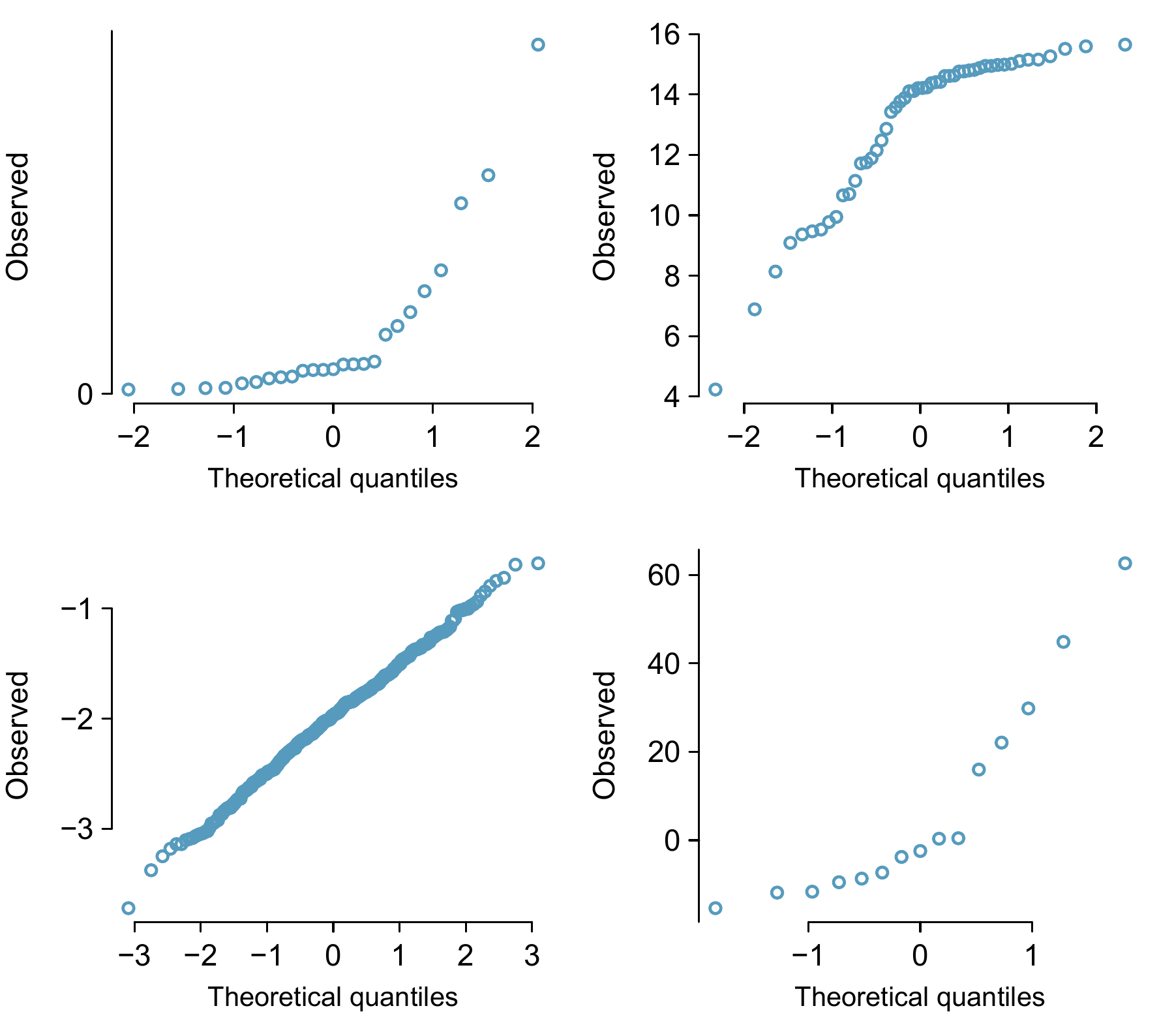
Figure 8.10: Four normal probability plots for Guided Practice 8.17.

When observations spike downwards on the left side of a normal probability plot, it means the data have more outliers in the left tail than we’d expect under a normal distribution. When observations spike upwards on the right side, it means the data have more outliers in the right tail than what we’d expect under the normal distribution.

Guided Practice8.18 Figure 8.11 shows normal probability plots for two distributions that are skewed. One distribution is skewed to the low end (left skewed) and the other to the high end (right skewed). Which is which?⁷¹

Figure 8.11: Normal probability plots for Guided Practice 8.18.

8.3 Geometric Distribution

How long should we expect to flip a coin until it turns up \(heads\)? Or how many times should we expect to roll a die until we get a \(1\)? These questions can be answered using the geometric distribution. We first formalize each trial – such as a single coin flip or die toss – using the Bernoulli distribution, and then we combine these with our tools from probability (Chapter 7) to construct the geometric distribution.

8.3.1 Bernoulli distribution

Stanley Milgram began a series of experiments in 1963 to estimate what proportion of people would willingly obey an authority and give severe shocks to a stranger. Milgram found that about 65% of people would obey the authority and give such shocks. Over the years, additional research suggested this number is approximately consistent across communities and time.⁷²

Each person in Milgram’s experiment can be thought of as a trial. We label a person a success if she refuses to administer the worst shock. A person is labelled a failure if she administers the worst shock. Because only 35% of individuals refused to administer the most severe shock, we denote the probability of a success with \(p=0.35\). The probability of a failure is sometimes denoted with \(q=1-p\).

Thus, success or failure is recorded for each person in the study. When an individual trial only has two possible outcomes, it is called a Bernoulli random variable.

Definition 8.3 (Bernoulli random variable, descriptive) A Bernoulli random variable has exactly two possible outcomes. We typically label one of these outcomes a “success” and the other outcome a “failure.” We may also denote a success by \(1\) and a failure by \(0\).

Remark (“success” need not be something positive). We chose to label a person who refuses to administer the worst shock a “success” and all others as “failures.” However, we could just as easily have reversed these labels. The mathematical framework we will build does not depend on which outcome is labelled a success and which a failure, as long as we are consistent.

Bernoulli random variables are often denoted as \(1\) for a success and \(0\) for a failure. In addition to being convenient in entering data, it is also mathematically handy. Suppose we observe ten trials: \[ 0\ 1\ 1\ 1\ 1\ 0\ 1\ 1\ 0\ 0 \] Then the sample proportion, \(\hat{p}\), is the sample mean of these observations: \[ \hat{p} = \frac{\#\text{ of successes}}{\#\text{ of trials}} = \frac{0+1+1+1+1+0+1+1+0+0}{10} = 0.6 \] This mathematical inquiry of Bernoulli random variables can be extended even further. Because \(0\) and \(1\) are numerical outcomes, we can define the mean and standard deviation of a Bernoulli random variable.⁷³

Definition 8.4 (Bernoulli random variable, mathematical) If \(X\) is a random variable that takes value \(1\) with probability of success \(p\) and \(0\) with probability \(1-p\), then \(X\) is a Bernoulli random variable with mean and standard deviation \[ \begin{aligned} \mu &= p &\sigma&= \sqrt{p(1-p)} \end{aligned} \]

In general, it is useful to think about a Bernoulli random variable as a random process with only two outcomes: a success or failure. Then we build our mathematical framework using the numerical labels \(1\) and \(0\) for successes and failures, respectively.

8.3.2 Geometric distribution

Example 8.10 Dr. Smith wants to repeat Milgram’s experiments but she only wants to sample people until she finds someone who will not inflict the worst shock.⁷⁴ If the probability a person will not give the most severe shock is still 0.35 and the subjects are independent, what are the chances that she will stop the study after the first person? The second person? The third? What about if it takes her \(n-1\) individuals who will administer the worst shock before finding her first success, i.e. the first success is on the \(n^{th}\) person? (If the first success is the fifth person, then we say \(n=5\).)

The probability of stopping after the first person is just the chance the first person will not administer the worst shock: \(1-0.65=0.35\). The probability it will be the second person is \[ \begin{aligned} &P(\text{second person is the first to not administer the worst shock}) \\ &\quad = P(\text{the first will, the second won't}) = (0.65)(0.35) = 0.228 \end{aligned} \]

Likewise, the probability it will be the third person is \((0.65)(0.65)(0.35) = 0.148\).

If the first success is on the \(n^{th}\) person, then there are \(n-1\) failures and finally 1 success, which corresponds to the probability \((0.65)^{n-1}(0.35)\). This is the same as \((1-0.35)^{n-1}(0.35)\).

Example 8.10 illustrates what is called the geometric distribution, which describes the waiting time until a success for independent and identically distributed (iid) Bernoulli random variables. In this case, the independence aspect just means the individuals in the example don’t affect each other, and identical means they each have the same probability of success.

The geometric distribution from Example 8.10 is shown in Figure 8.12. In general, the probabilities for a geometric distribution decrease exponentially fast.

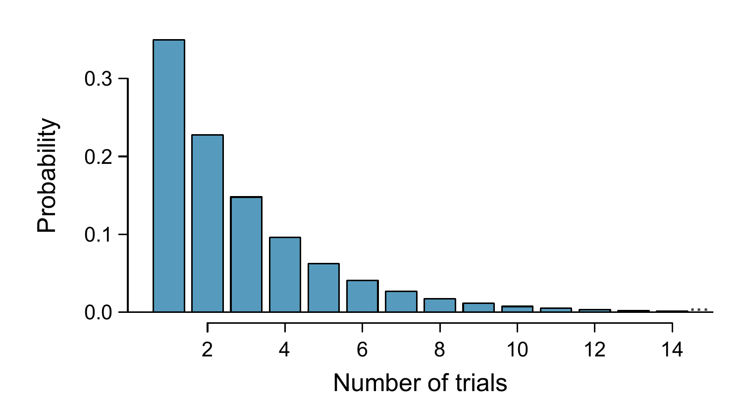
Figure 8.12: The geometric distribution when the probability of success is \(p=0.35\).

While this text will not derive the formulas for the mean (expected) number of trials needed to find the first success or the standard deviation or variance of this distribution, we present general formulas for each.

Definition 8.5 (Geometric Distribution) If the probability of a success in one trial is \(p\) and the probability of a failure is \(1-p\), then the probability of finding the first success in the \(n^{th}\) trial is given by \[ (1-p)^{n-1}p \] The mean (i.e. expected value), variance, and standard deviation of this wait time are given by \[ \begin{aligned} \mu &= \frac{1}{p} &\sigma^2&=\frac{1-p}{p^2} &\sigma &= \sqrt{\frac{1-p}{p^2}} \end{aligned} \tag{8.1} \]

It is no accident that we use the symbol \(\mu\) for both the mean and expected value. The mean and the expected value are one and the same.

The left side of Equation (8.1) says that, on average, it takes \(1/p\) trials to get a success. This mathematical result is consistent with what we would expect intuitively. If the probability of a success is high (e.g. 0.8), then we don’t usually wait very long for a success: \(1/0.8 = 1.25\) trials on average. If the probability of a success is low (e.g. 0.1), then we would expect to view many trials before we see a success: \(1/0.1 = 10\) trials.

Guided Practice8.19 The probability that an individual would refuse to administer the worst shock is said to be about 0.35. If we were to examine individuals until we found one that did not administer the shock, how many people should we expect to check? The first expression in Equation (8.1) may be useful.⁷⁵

Example 8.11 What is the chance that Dr. Smith will find the first success within the first 4 people?

This is the chance it is the first (\(n=1\)), second (\(n=2\)), third (\(n=3\)), or fourth (\(n=4\)) person as the first success, which are four disjoint outcomes. Because the individuals in the sample are randomly sampled from a large population, they are independent. We compute the probability of each case and add the separate results: \[ \begin{aligned} &P(n=1, 2, 3,\text{ or }4) \\ & \quad = P(n=1)+P(n=2)+P(n=3)+P(n=4) \\ & \quad = (0.65)^{1-1}(0.35) + (0.65)^{2-1}(0.35) + (0.65)^{3-1}(0.35) + (0.65)^{4-1}(0.35) \\ & \quad = 0.82 \end{aligned} \] There is an 82% chance that she will end the study within 4 people.

Guided Practice8.20 Determine a more clever way to solve Example 8.11. Show that you get the same result.⁷⁶

Example 8.12 Suppose in one region it was found that the proportion of people who would administer the worst shock was “only” 55%. If people were randomly selected from this region, what is the expected number of people who must be checked before one was found that would be deemed a success? What is the standard deviation of this waiting time?

A success is when someone will inflict the worst shock, which has probability \(p=1-0.55=0.45\) for this region. The expected number of people to be checked is \(1/p = 1/0.45 = 2.22\) and the standard deviation is \(\sqrt{(1-p)/p^2} = 1.65\).

Guided Practice8.21 Using the results from Example 8.12, \(\mu = 2.22\) and \(\sigma = 1.65\), would it be appropriate to use the normal model to find what proportion of experiments would end in 3 or fewer trials?⁷⁷

The independence assumption is crucial to the geometric distribution’s accurate description of a scenario. Mathematically, we can see that to construct the probability of the success on the \(n^{th}\) trial, we had to use the Multiplication Rule for Independent Processes. It is no simple task to generalize the geometric model for dependent trials.

8.4 Binomial Distribution

Example 8.13 Suppose we randomly selected four individuals to participate in the “shock” study. What is the chance exactly one of them will be a success? Let’s call the four people Allen (\(A\)), Brittany (\(B\)), Caroline (\(C\)), and Damian (\(D\)) for convenience. Also, suppose 35% of people are successes as in the previous version of this example.

Let’s consider a scenario where one person refuses: \[ \begin{aligned} &P(A=\texttt{refuse},\text{ }B=\texttt{shock},\text{ }C=\texttt{shock},\text{ }D=\texttt{shock}) \\ &\quad = P(A=\texttt{refuse})\ P(B=\texttt{shock})\ P(C=\texttt{shock})\ P(D=\texttt{shock}) \\ &\quad = (0.35) (0.65) (0.65) (0.65) = (0.35)^1 (0.65)^3 = 0.096 \end{aligned} \] But there are three other scenarios: Brittany, Caroline, or Damian could have been the one to refuse. In each of these cases, the probability is again \((0.35)^1(0.65)^3\). These four scenarios exhaust all the possible ways that exactly one of these four people could refuse to administer the most severe shock, so the total probability is \(4\times(0.35)^1(0.65)^3 = 0.38\).

Guided Practice8.22 Verify that the scenario where Brittany is the only one to refuse to give the most severe shock has probability \((0.35)^1(0.65)^3\).⁷⁸

8.4.1 The binomial distribution

The scenario outlined in Example 8.13 is a special case of what is called the binomial distribution. The binomial distribution describes the probability of having exactly \(k\) successes in \(n\) independent Bernoulli trials with probability of a success \(p\) (in Example 8.13, \(n=4\), \(k=1\), \(p=0.35\)). We would like to determine the probabilities associated with the binomial distribution more generally, i.e. we want a formula where we can use \(n\), \(k\), and \(p\) to obtain the probability. To do this, we reexamine each part of the example.

There were four individuals who could have been the one to refuse, and each of these four scenarios had the same probability. Thus, we could identify the final probability as \[ [\#\text{ of scenarios}] \times P(\text{single scenario}) \tag{8.2} \] The first component of this equation is the number of ways to arrange the \(k=1\) successes among the \(n=4\) trials. The second component is the probability of any of the four (equally probable) scenarios.

Consider \(P(\)single scenario\()\) under the general case of \(k\) successes and \(n-k\) failures in the \(n\) trials. In any such scenario, we apply the Multiplication Rule for independent events: \[ p^k(1-p)^{n-k} \] This is our general formula for \(P(\)single scenario\()\).

Secondly, we introduce a general formula for the number of ways to choose \(k\) successes in \(n\) trials, i.e. arrange \(k\) successes and \(n-k\) failures: \[ {n\choose k} = \frac{n!}{k!(n-k)!} \] The quantity \({n\choose k}\) is read n choose k.⁷⁹ The exclamation mark notation (e.g. \(k!\)) denotes a factorial expression. \[ \begin{aligned} & 0! = 1 \\ & 1! = 1 \\ & 2! = 2\times1 = 2 \\ & 3! = 3\times2\times1 = 6 \\ & 4! = 4\times3\times2\times1 = 24 \\ & \vdots \\ & n! = n\times(n-1)\times...\times3\times2\times1 \end{aligned} \tag{8.3} \] Using the formula, we can compute the number of ways to choose \(k=1\) successes in \(n=4\) trials: \[ {4 \choose 1} = \frac{4!}{1!(4-1)!} = \frac{4!}{1!3!} = \frac{4\times3\times2\times1}{(1)(3\times2\times1)} = 4 \] This result is exactly what we found by carefully thinking of each possible scenario in Example 8.13.

Substituting \(n\) choose \(k\) for the number of scenarios and \(p^k(1-p)^{n-k}\) for the single scenario probability in Equation (8.2) yields the general binomial formula.

Definition 8.6 (Binomial distribution) Suppose the probability of a single trial being a success is \(p\). Then the probability of observing exactly \(k\) successes in \(n\) independent trials is given by \[ {n\choose k}p^k(1-p)^{n-k} = \frac{n!}{k!(n-k)!}p^k(1-p)^{n-k} \tag{8.4} \] Additionally, the mean, variance, and standard deviation of the number of observed successes are \[ \begin{aligned} \mu &= np\\ \sigma^2 &= np(1-p)\\ \sigma &= \sqrt{np(1-p)} \end{aligned} \tag{8.5} \]

Remark (Is it binomial? Four conditions to check.).  

1. The trials are independent.
   
2. The number of trials, \(n\), is fixed.
   
3. Each trial outcome can be classified as a success or failure.
   
4. The probability of a success, \(p\), is the same for each trial.

Example 8.14 What is the probability that 3 of 8 randomly selected students will refuse to administer the worst shock, i.e. 5 of 8 will?

We would like to apply the binomial model, so we check our conditions. The number of trials is fixed (\(n=8\)) (condition 2) and each trial outcome can be classified as a success or failure (condition 3). Because the sample is random, the trials are independent (condition 1) and the probability of a success is the same for each trial (condition 4).

In the outcome of interest, there are \(k=3\) successes in \(n=8\) trials, and the probability of a success is \(p=0.35\). So the probability that 3 of 8 will refuse is given by \[ \begin{aligned} { 8 \choose 3}(0.35)^3(1-0.35)^{8-3} =& \frac{8!}{3!(8-3)!}(0.35)^3(1-0.35)^{8-3} \\ =& \frac{8!}{3!5!}(0.35)^3(0.65)^5 \end{aligned} \]

Dealing with the factorial part: \[ \frac{8!}{3!5!} = \frac{8\times7\times6\times5\times4\times3\times2\times1}{(3\times2\times1)(5\times4\times3\times2\times1)} = \frac{8\times7\times6}{3\times2\times1} = 56 \] Using \((0.35)^3(0.65)^5 \approx 0.005\), the final probability is about \(56\times 0.005 = 0.28\).

Remark (computing binomial probabilities). The first step in using the binomial model is to check that the model is appropriate. The second step is to identify \(n\), \(p\), and \(k\). The final step is to apply the formulas and interpret the results.

Remark (computing n choose k). In general, it is useful to do some cancellation in the factorials immediately. Alternatively, many computer programs and calculators have built in functions to compute \(n\) choose \(k\), factorials, and even entire binomial probabilities.

Guided Practice8.23 If you ran a study and randomly sampled 40 students, how many would you expect to refuse to administer the worst shock? What is the standard deviation of the number of people who would refuse? Equation (8.5) may be useful.⁸⁰

Guided Practice8.24 The probability that a random smoker will develop a severe lung condition in his or her lifetime is about \(0.3\). If you have 4 friends who smoke, are the conditions for the binomial model satisfied?⁸¹

Guided Practice8.25 Suppose these four friends do not know each other and we can treat them as if they were a random sample from the population. Is the binomial model appropriate? What is the probability that

1. none of them will develop a severe lung condition?
   
2. One will develop a severe lung condition?
   
3. That no more than one will develop a severe lung condition?⁸²

Guided Practice8.26 What is the probability that at least 2 of your 4 smoking friends will develop a severe lung condition in their lifetimes?⁸³

Guided Practice8.27 Suppose you have 7 friends who are smokers and they can be treated as a random sample of smokers.

1. How many would you expect to develop a severe lung condition, i.e. what is the mean?
   
2. What is the probability that at most 2 of your 7 friends will develop a severe lung condition.⁸⁴

Next we consider the first term in the binomial probability, \(n\) choose \(k\) under some special scenarios.

Guided Practice8.28 Why is it true that \({n \choose 0}=1\) and \({n \choose n}=1\) for any number \(n\)?⁸⁵

Guided Practice8.29  

• How many ways can you arrange one success and \(n-1\) failures in \(n\) trials?
  
• How many ways can you arrange \(n-1\) successes and one failure in \(n\) trials?⁸⁶

8.4.2 Normal approximation to the binomial distribution

The binomial formula is cumbersome when the sample size (\(n\)) is large, particularly when we consider a range of observations. In some cases we may use the normal distribution as an easier and faster way to estimate binomial probabilities.

Example 8.15 Approximately 14.5% of the Australian adult population smokes cigarettes.⁸⁷ A local government believed their community had a lower smoker rate and commissioned a survey of 400 randomly selected individuals. The survey found that only 39 of the 400 participants smoke cigarettes. If the true proportion of smokers in the community was really 14.5%, what is the probability of observing 39 or fewer smokers in a sample of 400 people? We leave the usual verification that the four conditions for the binomial model are valid as an exercise.

The question posed is equivalent to asking, what is the probability of observing \(k=0\), 1, …, 38, or 39 smokers in a sample of \(n=400\) when \(p=0.145\)? We can compute these 40 different probabilities and add them together to find the answer: \[ \begin{aligned} &P(k=0\text{ or }k=1\text{ or }\cdots\text{ or } k=39) \\ &\qquad= P(k=0) + P(k=1) + \cdots + P(k=39) \\ &\qquad=0.0030 \end{aligned} \] If the true proportion of smokers in the community is \(p=0.145\), then the probability of observing 39 or fewer smokers in a sample of \(n=400\) is 0.0030. In R this can be calculated as follows:

# calculate the probability P(X<=39) when X has Bin(n=400, p=0.145) distribution
pbinom(q = 39, size = 400, prob = 0.145, lower.tail = TRUE)
#> [1] 0.00303

Although the once tedious computation in Example 8.15 is now easily performed using the software, there are still occasions when calculating the exact binomial probabilities is best avoided. We might wonder, is it reasonable to use the normal model in place of the binomial distribution? Surprisingly, yes, if certain conditions are met.

Guided Practice8.30 Here we consider the binomial model when the probability of a success is \(p=0.10\). Figure 8.13 shows four hollow histograms for simulated samples from the binomial distribution using four different sample sizes: \(n=10, 30, 100, 300\). What happens to the shape of the distributions as the sample size increases? What distribution does the last hollow histogram resemble?⁸⁸

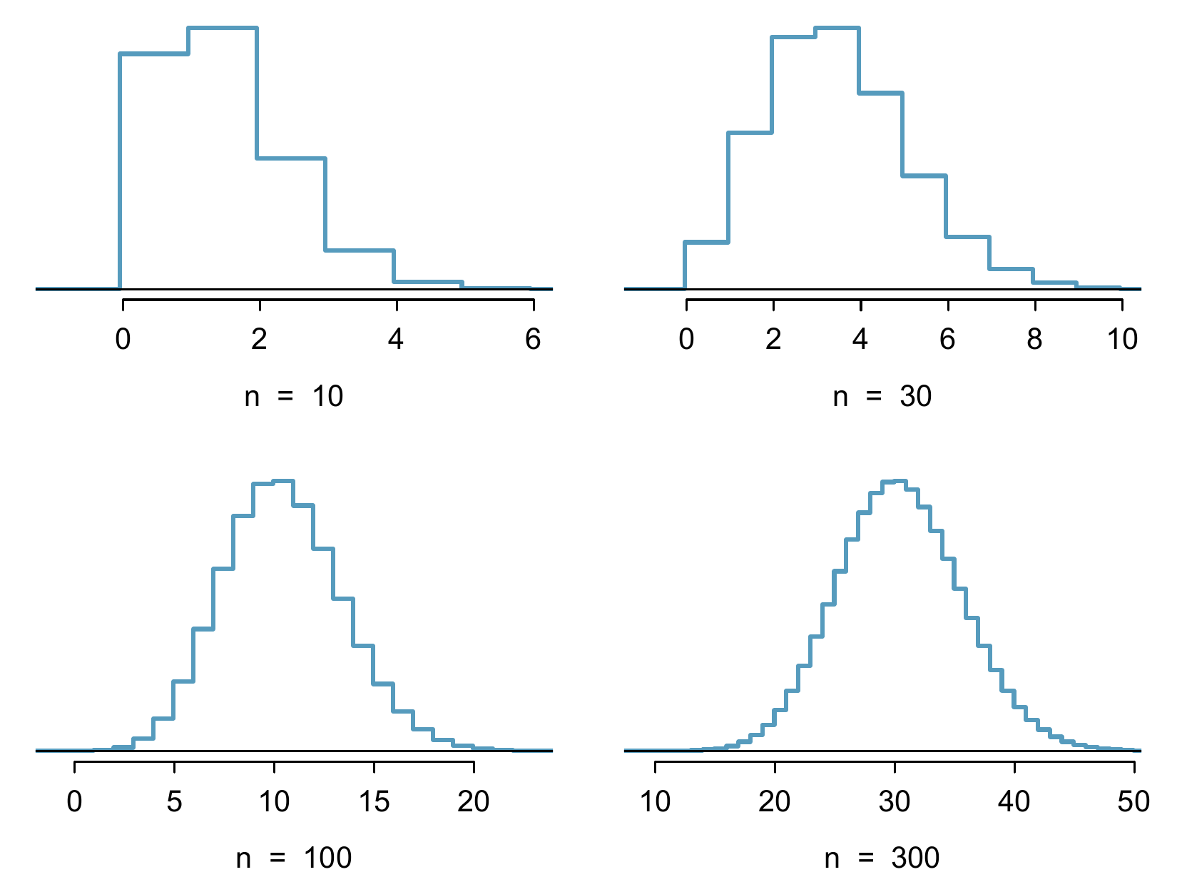
Figure 8.13: Hollow histograms of samples from the binomial model when \(p=0.10\). The sample sizes for the four plots are \(n=10\), 30, 100, and 300, respectively.

Definition 8.7 (Normal approximation of the binomial distribution) The binomial distribution with probability of success \(p\) is nearly normal when the sample size \(n\) is sufficiently large that \(np\) and \(n(1-p)\) are both at least 10. The approximate normal distribution has parameters corresponding to the mean and standard deviation of the binomial distribution: \[ \begin{aligned} \mu &= np\\ \sigma&= \sqrt{np(1-p)} \end{aligned} \]

The normal approximation may be used when computing the range of many possible successes. For instance, we may apply the normal distribution to the setting of Example 8.15.

Example 8.16 How can we use the normal approximation to estimate the probability of observing 39 or fewer smokers in a sample of 400, if the true proportion of smokers is \(p=0.145\)?

Showing that the binomial model is reasonable was a suggested exercise in Example 8.15. We also verify that both \(np\) and \(n(1-p)\) are at least 10: \[ \begin{aligned} np&=400\times 0.145=58\\ n(1-p)&=400\times 0.855=342 \end{aligned} \] With these conditions checked, we may use the normal approximation in place of the binomial distribution using the mean and standard deviation from the binomial model: \[ \begin{aligned} \mu &= np = 58\\ \sigma &= \sqrt{np(1-p)} = 7.04 \end{aligned} \] We want to find the probability of observing fewer than 39 smokers using this model.

Guided Practice8.31 Use the normal model \(N(\mu=58, \sigma=7.04)\) to estimate the probability of observing fewer than 39 smokers. Your answer should be approximately equal to the solution of Example 8.15: 0.0030.⁸⁹

---

50. It is also introduced as the Gaussian distribution after Carl Friedrich Gauss, the first person to formalize its mathematical expression.↩︎

51. (a) \(N(\mu=5,\sigma=3)\). (b) \(N(\mu=-100, \sigma=10)\). (c) \(N(\mu=2, \sigma=9)\).↩︎

52. \(Z_{Tom} = \frac{x_{Tom} - \mu_{ACT}}{\sigma_{ACT}} = \frac{24 - 21}{5} = 0.6\)↩︎

53. (a) Its \(Z\)-score is given by \(Z = \frac{x-\mu}{\sigma} = \frac{5.19 - 3}{2} = 2.19/2 = 1.095\). (b) The observation \(x\) is 1.095 standard deviations above the mean. We know it must be above the mean since \(Z\) is positive.↩︎

54. For \(x_1=95.4\) mm: \(Z_1 = \frac{x_1 - \mu}{\sigma} = \frac{95.4 - 92.6}{3.6} = 0.78\). For \(x_2=85.8\) mm: \(Z_2 = \frac{85.8 - 92.6}{3.6} = -1.89\).↩︎

55. Because the absolute value of \(Z\)-score for the second observation is larger than that of the first, the second observation has a more unusual head length.↩︎

56. If 84% had lower scores than Ann, the proportion of people who had better scores must be 16%. (Generally ties are ignored when the normal model, or any other continuous distribution, is used.)↩︎

57. We found the probability in Example 8.2: 0.6664. A picture for this exercise is represented by the shaded area below “0.6664” in Example 8.2.↩︎

58. If Edward did better than 37% of SAT takers, then about 63% must have done better than him. ↩︎

59. Numerical answers: (a) 0.9772. (b) 0.0228.↩︎

60. This sample was taken from the USDA Food Commodity Intake Database.↩︎

61. First put the heights into inches: 67 and 76 inches. Figures are shown below. (a) \(Z_{Mike} = \frac{67 - 70}{3.3} = -0.91\ \to\ 0.1814\). (b) \(Z_{Jim} = \frac{76 - 70}{3.3} = 1.82\ \to\ 0.9656\). ↩︎

62. Remember: draw a picture first, then find the \(Z\)-score. (We leave the pictures to you.) The \(Z\)-score can be found by using the percentiles and the normal probability table. (a) We look for 0.95 in the probability portion (middle part) of the normal probability table, which leads us to row 1.6 and (about) column 0.05, i.e. \(Z_{95}=1.65\). Knowing \(Z_{95}=1.65\), \(\mu = 1500\), and \(\sigma = 300\), we setup the \(Z\)-score formula: \(1.65 = \frac{x_{95} - 1500}{300}\). We solve for \(x_{95}\): \(x_{95} = 1995\). (b) Similarly, we find \(Z_{97.5} = 1.96\), again setup the \(Z\)-score formula for the heights, and calculate \(x_{97.5} = 76.5\).↩︎

63. Numerical answers: (a) 0.1131. (b) 0.3821.↩︎

64. This is an abbreviated solution. (Be sure to draw a figure!) First find the percent who get below 1500 and the percent that get above 2000: \(Z_{1500} = 0.00 \to 0.5000\) (area below), \(Z_{2000} = 1.67 \to 0.0475\) (area above). Final answer: \(1.0000-0.5000 - 0.0475 = 0.4525\).↩︎

65. 5’5’’ is 65 inches. 5’7’’ is 67 inches. Numerical solution: \(1.000 - 0.0649 - 0.8183 = 0.1168\), i.e. 11.68%.↩︎

66. First draw the pictures. To find the area between \(Z=-1\) and \(Z=1\), use the normal probability table to determine the areas below \(Z=-1\) and above \(Z=1\). Next verify the area between \(Z=-1\) and \(Z=1\) is about 0.68. Repeat this for \(Z=-2\) to \(Z=2\) and also for \(Z=-3\) to \(Z=3\).↩︎

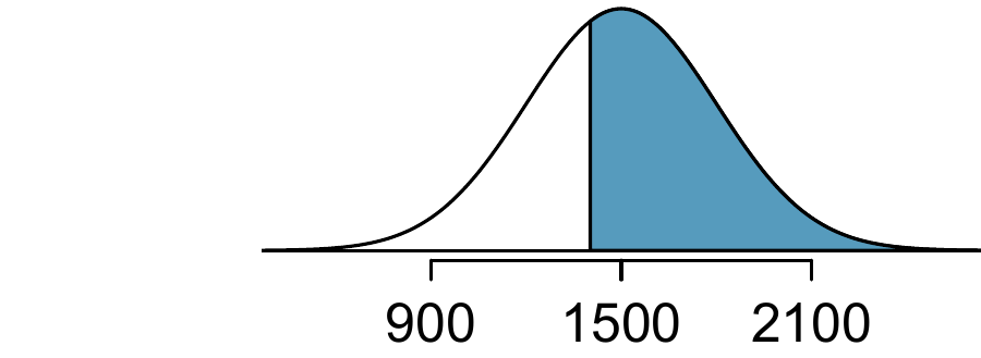
67. (a) 900 and 2100 represent two standard deviations above and below the mean, which means about 95% of test takers will score between 900 and 2100. (b) Since the normal model is symmetric, then half of the test takers from part (a) (\(\frac{95\%}{2} = 47.5\%\) of all test takers) will score 900 to 1500 while 47.5% score between 1500 and 2100.↩︎

68. Also commonly called a quantile-quantile plot or Q-Q plot↩︎

69. These data were collected from www.nba.com.↩︎

70. Answers may vary a little. The top-left plot shows some deviations in the smallest values in the data set; specifically, the left tail of the data set has some outliers we should be wary of. The top-right and bottom-left plots do not show any obvious or extreme deviations from the lines for their respective sample sizes, so a normal model would be reasonable for these data sets. The bottom-right plot has a consistent curvature that suggests it is not from the normal distribution. If we examine just the vertical coordinates of these observations, we see that there is a lot of data between -20 and 0, and then about five observations scattered between 0 and 70. This describes a distribution that has a strong right skew.↩︎

71. Examine where the points fall along the vertical axis. In the first plot, most points are near the low end with fewer observations scattered along the high end; this describes a distribution that is skewed to the high end. The second plot shows the opposite features, and this distribution is skewed to the low end.↩︎

72. Find further information on Milgram’s experiment at www.cnr.berkeley.edu/ucce50/ag-labor/7article/article35.htm.↩︎

73. If \({p}\) is the true probability of a success, then the mean of a Bernoulli random variable \(X\) is given by \[ \begin{aligned} \mu = E[X] &= P(X=0)\times0 + P(X=1)\times1 \\ &= (1-p)\times0 + p\times 1 = 0+p = p \end{aligned} \] Similarly, the variance of \(X\) can be computed: \[ \begin{aligned} \sigma^2 &= {P(X=0)(0-p)^2 + P(X=1)(1-p)^2} \\ &= {(1-p)p^2 + p(1-p)^2} = {p(1-p)} \end{aligned} \] The standard deviation is \(\sigma=\sqrt{p(1-p)}\).↩︎

74. This is hypothetical since, in reality, this sort of study probably would not be permitted any longer under current ethical standards.↩︎

75. We would expect to see about \(1/0.35 = 2.86\) individuals to find the first success.↩︎

76. First find the probability of the complement: \(P(\)no success in first 4~trials\() = 0.65^4 = 0.18\). Next, compute one minus this probability: \(1-P(\)no success in 4 trials\() = 1-0.18 = 0.82\).↩︎

77. No. The geometric distribution is always right skewed and can never be well-approximated by the normal model.↩︎

78. \(P(A=\texttt{shock},\text{ }B=\texttt{refuse},\text{ }C=\texttt{shock},\text{ }D=\texttt{shock}) = (0.65)(0.35)(0.65)(0.65) = (0.35)^1(0.65)^3\).↩︎

79. Other notation for \(n\) choose \(k\) includes \(_nC_k\), \(C_n^k\), and \(C(n,k)\).↩︎

80. We are asked to determine the expected number (the mean) and the standard deviation, both of which can be directly computed from the formulas in Equation (8.5): \(\mu=np = 40\times 0.35 = 14\) and \(\sigma = \sqrt{np(1-p)} = \sqrt{40\times 0.35\times 0.65} = 3.02\). Because very roughly 95% of observations fall within 2 standard deviations of the mean, we would probably observe at least 8 but less than 20 individuals in our sample who would refuse to administer the shock.↩︎

81. One possible answer: if the friends know each other, then the independence assumption is probably not satisfied. For example, acquaintances may have similar smoking habits.↩︎

82. To check if the binomial model is appropriate, we must verify the conditions. (i) Since we are supposing we can treat the friends as a random sample, they are independent. (ii) We have a fixed number of trials (\(n=4\)). (iii) Each outcome is a success or failure. (iv) The probability of a success is the same for each trials since the individuals are like a random sample (\(p=0.3\) if we say a “success” is someone getting a lung condition, a morbid choice). Compute parts (a) and (b) from the binomial formula in Equation (8.4): \(P(0) = {4 \choose 0} (0.3)^0 (0.7)^4 = 1\times1\times0.7^4 = 0.2401\), \(P(1) = {4 \choose 1} (0.3)^1(0.7)^{3} = 0.4116\). Note: \(0!=1\). Part (c) can be computed as the sum of parts (a) and (b): \(P(0) + P(1) = 0.2401 + 0.4116 = 0.6517\). That is, there is about a 65% chance that no more than one of your four smoking friends will develop a severe lung condition.↩︎

83. The complement (no more than one will develop a severe lung condition) as computed in Guided Practice 8.25 as 0.6517, so we compute one minus this value: 0.3483.↩︎

84. (a) \(\mu=0.3\times7 = 2.1\). (b) \(P(0, 1,\text{ or }2\text{ develop severe lung condition}) = P(k=0) + P(k=1)+P(k=2) = 0.6471\).↩︎

85. Frame these expressions into words. How many different ways are there to arrange 0 successes and \(n\) failures in \(n\) trials? (1 way.) How many different ways are there to arrange \(n\) successes and 0 failures in \(n\) trials? (1 way.)↩︎

86. One success and \(n-1\) failures: there are exactly \(n\) unique places we can put the success, so there are \(n\) ways to arrange one success and \(n-1\) failures. A similar argument is used for the second question. Mathematically, we show these results by verifying the following two equations:\({n \choose 1} = n, \qquad {n \choose n-1} = n\)↩︎

87. http://www.abs.gov.au/AUSSTATS/abs@.nsf/DetailsPage/4364.0.55.0012014-15?OpenDocument ↩︎

88. The distribution is transformed from a blocky and skewed distribution into one that rather resembles the normal distribution in the last hollow histogram.↩︎

89. Compute the \(Z\)-score first: \(Z=\frac{39 - 58}{7.04} = -2.70\). The corresponding left tail area is 0.0035.↩︎