Chapter 18 Regression
Our focus is on fitting a trend line to observations. There are many different decision rules that could be used to decide how to fit the “best” trend line to a data set. The decision rule we will use to fit a trend line is to minimise the squared vertical distances between the trend line and the actual data points. We call the difference between where we fit the trend line and the actual data points the error term. In practical terms our decision rule means when we fit a trend line we try different intercept and different slope values until we get a line that fits the data as best as possible, where as best as possible means we have “minimised the sum of the squared error terms.”
The reason we minimise the squared error terms rather than just minimise the sum of the error terms is that sometimes the errors are positive and sometimes they are negative, so we need a decision rule that takes this into account. The two easiest solutions to the problem are to either take the absolute value of the error term or square the error term values. With either decision rule the error terms are all positive. For reasons of computational ease, the convention is to use squared error terms rather than the absolute value. This approach gives rise to the estimation method name: least squares estimation. If you fit a trend line using the sum of the absolute values of the error terms the approach is called least absolute deviation, but this second approach is but much less common than the method of least squares.
The general term used for the modelling approach of fitting a trend line to data is linear regression. Linear regression does not mean that we are always going to fit a straight line to the data, but fitting a straight line to the data will be our initial focus. Once the basic approach is mastered it is easy to extend the modelling approach to more complicated examples.
In the language of linear regression we say that the decision rule we use to fit the trend line is an estimator. So, we use the least squares estimator (decision rule) to obtain estimates of the slope and the intercept of the trend line. In linear regression the variable on the y-axis (vertical axis) is called the dependent variable or the response variable. The variable on the x-axis (horizontal axis) is called the explanatory variable or independent variable. Generally we think of the variable on the x-axis as being able to `explain’ the variable on the y-axis.
18.1 Estimating a Trend Line
In this example our data are the carapace sizes of lobsters at different distances to a no-take marine sanctuary. The research question is whether there is a relationship between lobster size and distance to the sanctuary. Specifically, we are interested in whether lobsters are smaller the further they are found from the no-take area.
We are not comparing lobster sizes at two difference distances, but rather we have data collected at a whole range of distances.
Let’s read in our data and have a look at it. Note that with grouped data we generally look at a boxplot, and with ungrouped data (a single numerical variable) we create a histogram or a horizontal boxplot. Here we are looking at the relationship rather than difference between two continuous (numerical) variables, so will create a scatter plot.
Note: There is a separate reference guide for scatter plots, so the descriptions given here are relatively brief.
Our \(\texttt{y}\) or dependent/response variable is lobster size, our \(\texttt{x}\) or independent/explanatory variable is distance to the no-take area (sanctuary). When plotting and creating linear regression models we give R the formula: \(\texttt{y}\sim\texttt{x}\). Deciding which variable goes on the y-axis and which variable goes on the x-axis is tricky. The convention is to use the variable that we think is doing the explaining on the horizontal (x-axis). Because we think that distance from the no-take zone might `explain’ carapace width, we place distance on the horizontal axis and carapace width on the vertical.
# read in our data
lobster.data<- data.frame(
  distance= c(0, 2, 3, 4, 4, 5, 6, 7, 9, 12, 18, 20, 20, 23, 24, 26, 27, 28, 30),
  size= c(116.89, 96.90, 120.97, 116.40, 89.86, 96.83, 116.18, 117.02, 79.03,
          69.86, 105.60, 68.12, 78.12, 69.86, 66.64, 62.11, 59.11, 59.94, 44.43))

# have a look at the str, summary to mkae sure we understand the data
str(lobster.data) # we have 2 numerical or continuous variables
#> 'data.frame':    19 obs. of  2 variables:
#>  $ distance: num  0 2 3 4 4 5 6 7 9 12 ...
#>  $ size    : num  116.9 96.9 121 116.4 89.9 ...
summary(lobster.data) # 6 number summary of both variables
#>     distance         size
#>  Min.   : 0.0   Min.   : 44.4
#>  1st Qu.: 4.5   1st Qu.: 67.4
#>  Median :12.0   Median : 79.0
#>  Mean   :14.1   Mean   : 86.0
#>  3rd Qu.:23.5   3rd Qu.:110.9
#>  Max.   :30.0   Max.   :121.0
Now, rather than a boxplot we create a scatter plot. Note the form of the scatter plot formula is \(\texttt{y}\sim\texttt{x}\) so we have size~distance in the plot formula. Also note that in your own plots you will just have the figure caption, not a figure caption and a figure title.
with(lobster.data, plot(size~distance,
     pch= 4, # controls the dot format used
     # write title on two lines ( use \n or return for a new line)
     main= "Lobster size in relation to distance to a
            no-take marine sanctuary",
     ylab= "Lobster carapace size (mm)",
     xlab= "Distance from santuary (m)",
     ylim= c(40,130), xlim= c(0,30), las= 1))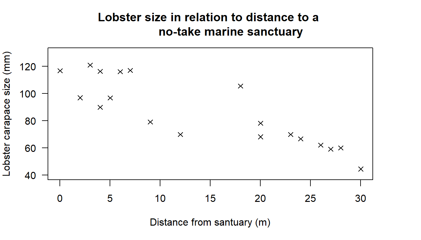
Figure 18.1: Scatter plot showing the relationship between distance to a no-take marine sanctuary and lobster carapace sizes.
What do you see here? Does there appear to be a linear relationship between the two variables, i.e. could you draw a straight line through the majority of the points? At the greatest distances from the sanctuary (25 - 30 m) we do see the smallest lobsters, and at the shortest distances (0 - 5 m) we have the largest lobsters, but in the middle values appear to be somewhat more random. The relationship is not perfect, but fitting a trend line to the data might help us understand what is going on.
Let’s add a trend line to the data by estimating a “linear” model with the function lm(), where lm stands for linear model. We will also save the model output as an object, giving it an intuitive name (lm.lobster) and calling on the data for the model using the parameter data.
Using the parameter data to indicate the data set we want R to use is a slight change in notation from the appraoch we have used for other models. For the ANOVA model, t-tests, Kruskal-Wallis test, and Wilcoxon test we used the with() command to tell R which data set to use.
To get the values for the trend line – the coefficients of the equation of the line - we use the function coef() calling on the model we created.
lm.lobster <- lm(size ~ distance, data = lobster.data)  # create our model
coef(lm.lobster)  # print our coefficients
#> (Intercept)    distance
#>      114.39       -2.01
Here we are given the values for our equation of the line: the intercept is 114.39 and slope for our explanatory variable (distance) is -2.01. Our slope is negative indicating we have a downward sloping trend. The reported intercept and slope values are the values that give a trend line that minimises the squared error terms between the actual data and the trend line.
As an equation this looks like: \(\texttt{fitted y-value = intercept + slope(x-data)}\)
Which we can write as: \(\texttt{y-hat = (114.388) + (-2.013)x}\)
Or in a clean general form: \(\hat{y} = 114.4 -2.0x\)
Or, in a form that makes clear what is being measured: \(\widehat{\texttt{size}} = 114.4 -2.0\times \texttt{Distance}.\)
The equation tells us that for every 1 m increase in distance from the no-take marine sanctuary, lobster carapace sizes decrease, on average, by about 2 mm. When we have a regression equation we always add the comment, on average. The intercept says that at \(0\)m away from the sanctuary lobster carapaces are estimated to be, on average, \(114\)mm. Because the data used to derive the model includes \(0\)m from the sanctuary, this can be considered a value that has some meaning. In most cases the intercept coefficient is not informative and so we will generally not look at the intercept term in our models.
Note: You have MUCH less confidence using a model to extrapolate beyond the range of your data. Formally we only know what is happening for the data range we observe. So, this model may be useful for predicting lobster size estimates from 0m to 121m from this sanctuary. Outside this range the model has little to say, and it would be dangerous to extrapolate.
The last step is to graphically display our model. We can do this by adding a trend line to our scatter plot with the abline() function and identifying our line in a legend with the legend() function. Note we can add the line either by specifying the numerical values directly (a = intercept and b = slope), or by telling R to get the slope and intercept from our model (m.lobster).
with(lobster.data, plot(size~distance,
     pch= 4,
     # write title on two lines ( use \n or return for a new line)
     main= "Lobster size in relation to distance to a
     no-take marine sanctuary",
     ylab= "Lobster carapace size (mm)",
     xlab= "Distance from santuary (m)",
     ylim= c(40,130), xlim= c(0,30), las= 1))

# add our trend line
abline(lm.lobster, lty= 2, lwd= 2, col= "blue")

# add our legend
legend("topright", legend= "trend line", lty= 2, lwd= 2, col= "blue", bty= "n")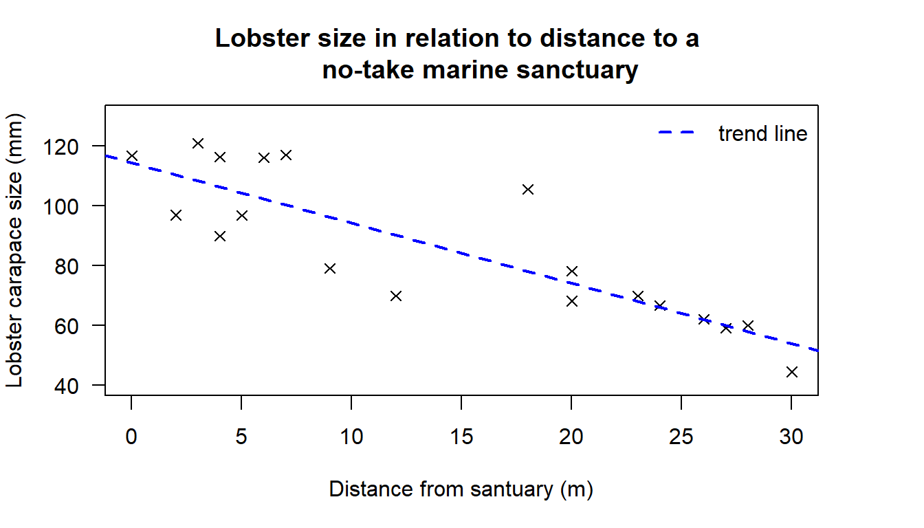
Figure 18.2: Scatter plot showing the relationship between distance to a no-take marine sanctuary and lobster carapace sizes, including linear model trend line
18.2 Statistical Significance of the Slope Estimate
The decision rule we use to generate an estimate of the slope and intercept (the least squares estimator) will always generate estimates of the slope and intercept. However, we are interested in knowing whether or not the slope estimate we obtain is statistically different from zero. The question we are asking is could the pattern we observe in the data be due to chance, or is it a real trend?
To determine whether or not the slope estimate is statistically different from zero we conduct a t-test. The t-test for the slope (and intercept) works the same way as our earlier t-tests, and we will use the same decision rule. Specifically, if the t-test p-value is less than 0.05 we will reject the null hypothesis that the slope estimate is equal to zero. In practice this decision rule means that we have set the test alpha level at 0.05.
To conduct the t-test we use the summary() function. The summary() function will conduct a t-test on both the slope and the intercept, and will also report some additional information on our linear model. This automated routine is one of the very useful things about R. While MS Excel will fit a trend line, the default output does not tell you whether or not the estimates are statistically different from zero. Let’s run a formal test on the model we created previously, and saved as: lm.lobster.
Step 1: Set the Null and Alternate Hypotheses
Here we will be testing only the slope as we are not interested in the intercept
- Null hypothesis: The slope is equal to zero
- Alternate hypothesis: The slope is not equal to zero
- Null hypothesis: The slope is equal to zero
Step 2: Print the test output
We obtain all the output with a simple command
summary(lm.lobster). The output we get has many elements but we will work through the detail in stages.summary(lm.lobster) # summary for our linear model #> #> Call: #> lm(formula = size ~ distance, data = lobster.data) #> #> Residuals: #> Min 1Q Median 3Q Max #> -20.371 -8.529 0.566 7.029 27.447 #> #> Coefficients: #> Estimate Std. Error t value Pr(>|t|) #> (Intercept) 114.388 5.133 22.28 5.1e-14 *** #> distance -2.013 0.296 -6.79 3.1e-06 *** #> --- #> Signif. codes: 0 '***' 0.001 '**' 0.01 '*' 0.05 '.' 0.1 ' ' 1 #> #> Residual standard error: 13 on 17 degrees of freedom #> Multiple R-squared: 0.731, Adjusted R-squared: 0.715 #> F-statistic: 46.1 on 1 and 17 DF, p-value: 3.15e-06Step 3: Interpret the Results
The output here is quite a bit more complex than for basic t-tests. Let’s focus, for now, on the “Coefficients” section of the output. This section of the output provides the estimates for our trend line and the results for the test of statistical significance. Under the “Estimate” column we see the same values as we obtained when using the
coef()function - the intercept and slope terms (distance is the slope estimate).The next column is the “Std. Error” column and the values in this column are the standard error for each coefficient. The standard error in a regression model has the same interpretation as the standard error of the mean in our earlier t-test examples. These values can be thought of as a measure of uncertainty for our slope and intercept values.
Next, we can see t-values. The t-values have been calculated using the approach we used for earlier t-tests. Specifically, these values have been calculated as: Estimate value minus the null hypothesis test value divided by the standard error. In this instance our null hypothesis test value is zero; so the t-value is calculated as: (-2.0131 - 0 / 0.2964) = -6.79. Lastly we can see the p-values. The p-values are what we use to make a decision about whether or not the slope estimate is statistically different from zero. Since the p-value for the slope is: \(\texttt{3.15e-06}\) \((< 0.001)\), which is smaller than \(0.05\), we: Reject the null hypothesis that the slope is equal to zero.
Why do we care if the slope estimate is different to zero? Well, if the slope is zero this means that there is no real trend in the data. The variation we have observed is just due to sampling variation. Fundamentally, we are interested in knowing whether the trend line we fit to the data represents a real trend line or not.
Another way to think about the null hypothesis for our test is that it asks the question: does a trend line fit the data better than a horizontal line at the mean of the data? A visual representation of the situation is given below. If the null were true, a horizontal line at the mean lobster carapace size would be a good description of the data. If the null is not true we are saying that a trend line fits the data better than a horizontal line. In our case, as we rejected the null, we are saying that the trend line is a better fit to the data than the horizontal line.
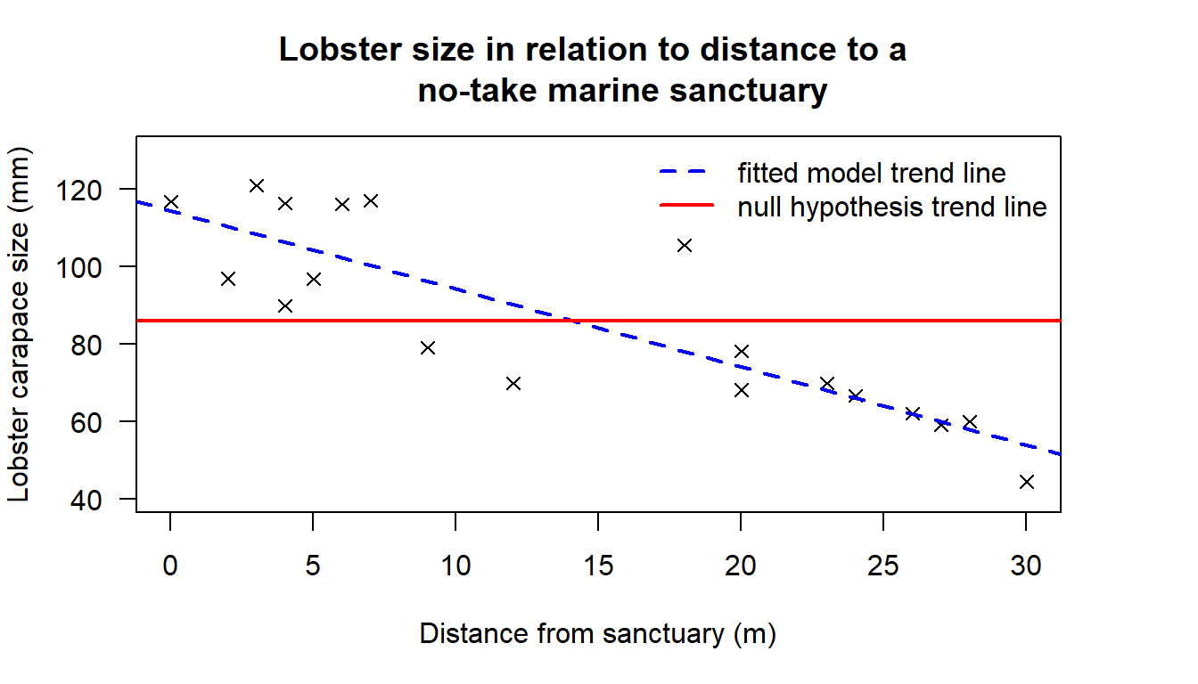
Figure 18.3: Scatter plot showing the relationship between distance to a no-take marine sanctuary and lobster carapace sizes.
18.3 Measure of Model Fit
Let’s again look at the model output. The final thing we are interested in is the \(R^2\) value. This value has an interpretation as the proportion of the variation in the data explained by the model. In R, the \(R^2\) value is reported as the Multiple R-squared value, which is the second last line of the summary output. See if you can find it in the output below.
summary(lm.lobster)  # provide model created previously
#>
#> Call:
#> lm(formula = size ~ distance, data = lobster.data)
#>
#> Residuals:
#>     Min      1Q  Median      3Q     Max
#> -20.371  -8.529   0.566   7.029  27.447
#>
#> Coefficients:
#>             Estimate Std. Error t value Pr(>|t|)
#> (Intercept)  114.388      5.133   22.28  5.1e-14 ***
#> distance      -2.013      0.296   -6.79  3.1e-06 ***
#> ---
#> Signif. codes:  0 '***' 0.001 '**' 0.01 '*' 0.05 '.' 0.1 ' ' 1
#>
#> Residual standard error: 13 on 17 degrees of freedom
#> Multiple R-squared:  0.731,  Adjusted R-squared:  0.715
#> F-statistic: 46.1 on 1 and 17 DF,  p-value: 3.15e-06
print(round(R_squared, 4))  # this is just to show you the value
#> [1] 0.731
# above is the R-squared value
As the \(R^2\) value = 0.731, we say that the model explains 73.1% of the variation in the data. We don’t really have a view regarding whether this is a good thing or a bad thing, but it is a commonly reported metric, and something that we will report.
There are other metrics of model fit, for example R also reports an Adjusted R-squared value. These other metrics do have advantages, but these alternative metrics do not have the same nice interpretation of percent/proportion of the variation in the data explained by the model. For this reason we will stick with reporting the \(R^2\) value.
18.4 The Summary Table
Because there are multiple t-tests (one for the intercept and one for the slope), and because there is additional information to report, such as the \(R^2\) value, the convention for reporting linear regression results in to use a summary table. The summary table contains:
- the estimates of the slope and the intercept;
- the standard error of the slope and the intercept, where a “*” sign is used to denote statistical significance;
- the number of observations in the data set; and
- the \(R^2\) value.
The difference between the estimate and the standard error is usually indicated with parentheses. Because it is possible to report either standard error information or t-value information, the convention is to add a footnote to the table to say “Standard errors in parentheses.” The thresholds chosen for statistical significance also vary.
Because we use p-value \(<0.05\) as the critical decision threshold for our t-tests, when we move to a more general system of critical thresholds we use alpha values around 0.05 that are both more and less stringent i.e. the threshold values we use for the “*” sign system of denoting statistical significance are “*” for p-value \(<0.1\); “**” for p-value \(<0.05\); “***” for p-value \(<0.01\).
Below is an example of an acceptable format for a regression summary table, but there are many other acceptable formats.
| Lobster size | |
| Intercept | 114.00*** (5.13) |
| Distance | -2.01*** (0.30) |
| Observations | 19 |
| R2 | 0.73 |
| Note: | p<0.1; p<0.05; p<0.01 |
| Standard errors in parentheses. | |