Chapter 20 Nonparametric Methods
The statistical inference methods that we have seen so far can be classed as parametric methods. We have an understanding of the the theoretical properties of different distributions of random variables. These distributions are defined by their parametric form: the Normal distribution has a mean and a variance; the \(t\)-distribution is defined by its mean and degrees of freedom. We then make assumptions about the underlying structure of the data we observe or about the population from which the data are drawn in order to make use of these distributions, and we make inference about the parameters of the distribution.
If we are not so sure that these parametric assumptions hold, we may prefer methods that are valid without such assumptions: non-parametric methods. These methods are robust to mis-specification of the underlying distribution of the data because they do not assume a particular distribution in the first place.
Non-parametric methods have long been used to establish whether or not two or more groups are the same. The tests work by first ranking the data and then using the rank values, not the actual data values. For this reason the tests are sometimes referred to as robust tests: the tests are robust to the influence of outliers. The situation is analogous to the comparison of the mean and the median. To find the median we rank the data from highest to lowest and look at the middle value. The median is therefore referred to as a measure that is robust to the influence of outliers. This is in contrast to the mean, which can be influenced by outliers.
The difference between using the actual data for a test, and using the rank data can be understood with a simple example. Consider the set: \(10, 5, 15, 4, 7, 14, 79\). This set of numbers has one relatively extreme value, and this value has a strong effect on the mean but not the median. Specifically the mean is \(17.1\), which is greater than six of the seven numbers, while the median is \(10\).
Rather than use the raw data values, non-parametric methods convert the raw data into ranks first and then use the rank values in the test. The mapping of the raw data to rank values is shown in Table 1. The smallest value in the data set is \(4\) and so the value \(4\) is given a rank value of \(1\). The second smallest value in the data set is \(5\) and so the value \(5\) is given a rank value of \(2\). The process continues until we get to the largest value in the data set, which is \(79\), and \(79\) is given a rank value of \(7\).
| Raw data values | 10 | 5 | 15 | 4 | 7 | 14 | 79 |
| Data rank values | 4 | 2 | 6 | 1 | 3 | 5 | 7 |
If the assumptions of the parametric model are valid, then parametric methods have a greater ability to detect a difference, if a difference exists. For this reason we generally only use non-parametric methods when we can not appeal to the central limit theorem. Recall that the central limit theorem tells us that for large sample sizes, the distribution of the sample mean will tend towards a Mornal distribution. So we prefer non-parametric methods generally when we have small samples. Deciding when it is necessary to use a non-parametric approach is tricky, so we will leave that for now and just focus on making sure we understand how to implement the key non-parametric approaches.
As with all previous statistical tests, we will set the alpha level at 0.05.
20.1 Two Sample Non-Parametric Test: Mann-Whitney Test
Rather than testing whether two samples come from populations with different means (the mean being a parameter), a non-parametric approach tests whether two samples came from two populations with the same distribution, or different distributions. The key here is that we don’t make any assumption about what type of distributions we are dealing with, we only care about whether the distributions are the same or not.
Under the null hypothesis that the two samples are independent samples from the same distribution, we know what the probabilities are of a unit in one sample being higher or lower than the units in the other sample. The Mann-Whitney test compares these theoretical probabilities under the null hypothesis to the observed realisations of which units are higher or lower than others in the two samples. In this way we get a probability of having observed two samples at least as different as the two samples in front of us, if the null hypothesis were true. Thus, we have a p-value for the test of whether the two samples come from the same distribution or not.
For this example we use the same phytoremediation data used for the two sample t-test. Recall, phytoremediation is the use of plants for remediating contaminated soil and water, and plant species are selected based on their ability to uptake or stabilize specific contaminants at a site.
Here we will look at the efficiency of two crop plants (redbeet and barley) at removing cadmium from the top 20 cm of soil at a contaminated site. The data we have is the percent reduction of cadmium after one harvest. Because we only have 15 observations for each plant we decide to use a non-parametric test. Because we have two independent samples we use a Mann-Whitney two sample test. So that the example can be reproduced, below I type in the data. In general your first step in to read in the data from a .csv file not type the data directly into R.
# read in our data (wide format)
Cd.BeetBarley <- data.frame(
  redbeet = c(18, 5, 10, 8, 16, 12, 8, 8, 11, 5, 6, 8, 9, 21, 9),
  barley = c(8, 5, 10, 19, 15, 18, 11, 8, 9, 4, 5, 13, 7, 5, 7)
)

# check the data structure
str(Cd.BeetBarley)
#> 'data.frame':    15 obs. of  2 variables:
#>  $ redbeet: num  18 5 10 8 16 12 8 8 11 5 ...
#>  $ barley : num  8 5 10 19 15 18 11 8 9 4 ...

#  the structure information tells un we have two columns of data, and
#  that there are 15 observations in each group
Once we understand the data structure, and are confident the data has been read into R correctly, we then create a boxplot to look at the data. Remember, the boxplot is an essentially part of the process whether we are using a parametric test or a non-parametric test.
with(
  Cd.BeetBarley,
  boxplot(
    redbeet,
    barley,
    col = "lightgrey",
    main = "Phytoremediation Efficiency of Crop Plants",
    xlab = "Crop type",
    ylab = "Cadmium reduction (%)",
    names = c("Redbeet", "Barley"),
    ylim =  c(0, 25),
    las = 1,
    boxwex = 0.6
  )
)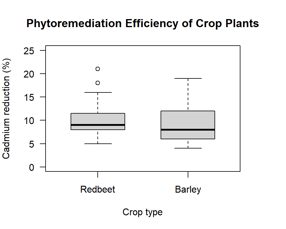
Figure 20.1: Box plot comparing the phytoremediation efficiency of redbeet and barley crop plants for removing cadmium from contaminated soil at depths of 0 to 20 cm.
Unlike the two sample t-test, for non-parametric tests there is no variance assumption to think about. We just jump straight to our main test for a difference between the groups. For non-parametric tests the statement about the null and the alternate hypothesis do not refer to the mean, but are just general statements.
Step 1: Set the Null and Alternate Hypotheses
Null hypothesis: The effectiveness of Redbeet and Barley in removing cadmium from the top 20cm of soil is the same
Alternate hypothesis: The effectiveness of Redbeet and Barley in removing cadmium from the top 20cm of soil is not the same.Step 2: Implement the test
We use thewilcox.test()function to implement the test, and the test notation is essentially the same as for thet.test()function. Although there is no equal/unequal variance parameter to set for the test, to suppress the warnings – which can be really annoying – when using the test we set the parameterexact = FALSE.with(Cd.BeetBarley, wilcox.test(redbeet, barley, exact = FALSE)) #> #> Wilcoxon rank sum test with continuity correction #> #> data: redbeet and barley #> W = 126, p-value = 0.6 #> alternative hypothesis: true location shift is not equal to 0 # use exact=FALSE to supress the warningsStep 3: Interpret the Results
From the output we see the $$0.573. Since 0.573 is greater than 0.05 (alpha), we:
Fail to reject the null hypothesis that the effectiveness of Redbeet and Barley in removing cadmium from the top 20cm of soil is the same.In other words: We do not have sufficient evidence to identify any kind of difference. If you were trying to determine which plant to use to remediate a particular site you would likely look to other factors, such as cost, environmental conditions or additional contaminants to be removed, to assist you in making your decision. Alternatively, you could think about collecting further data. With more data there is an increase in test power, and hence an increase in the ability to detect a difference if a difference exists.
20.2 Paired Non-Parametric Test: Wilcoxon Test
As with the Mann-Whitney test, the Wilcoxon test looks at pairs of observations and compares what is observed with what would be expected under the null hypothesis. The Wilcoxon test also makes use of the paired nature of the data, to test the null hypothesis that the the true distribution of the difference between observations is centered at zero and is symmetric. The difference we are talking about here is calculated for each individual in the sample, the difference of that individual’s observation under one condition minus the observation under the other.
This example is similar to the paired t-test example, and we will again be looking at before and after data from a contaminated site. Groundwater at the site was remediated using a Pump & Treat method with the intention of removing unacceptable levels of Total Petroleum Hydrocarbons (TPC). TCP is a general term encompassing hundreds of hydrocarbon based compounds. The paired measurements, recorded in micrograms per litre, were taken at observation wells around the contaminated site before and after the treatment.
We would like to determine whether the treatment has been effective - i.e. we want to determine whether or not there are differences between the measurements taken before and after the treatment. However, as we only have nine before and after measurements we decide we will use a non-parametric test rather than a paired t-test.
Generally you will read the data in from an MS Excel .csv file or similar, but here we input the data directly to provide a complete record of all the data needed for the test.
#test
# read in our data (wide format)
TPH.remediation <- data.frame(
  before = c(
    1475.7,
    1292.2,
    1575.9,
    1440.8,
    1606.1,
    1425.1,
    1502.3,
    1327.4,
    1526.4
  ),
  after = c(
    695.1,
    706.1,
    675.5,
    706.6,
    717.8,
    729.4,
    722.3,
    668.2,
    714.4
    )
  )

# Look at the raw data
str(TPH.remediation)
#> 'data.frame':    9 obs. of  2 variables:
#>  $ before: num  1476 1292 1576 1441 1606 ...
#>  $ after : num  695 706 676 707 718 ...
summary(TPH.remediation)
#>      before         after
#>  Min.   :1292   Min.   :668
#>  1st Qu.:1425   1st Qu.:695
#>  Median :1476   Median :707
#>  Mean   :1464   Mean   :704
#>  3rd Qu.:1526   3rd Qu.:718
#>  Max.   :1606   Max.   :729
With our data in R, we then move on to our standard process of analysis. The first step is a boxplot. Because we have paired data we are then going to create a horizontal boxplot of the difference in the observation pairs.
with(TPH.remediation,boxplot(before - after,
     col= "lightgray", boxwex= 1.2,
     main= "Pump and Treat Groundwater Remediation of
     Total Petroleum Hydrocarbons (TPH)",
     xlab= "Differences in TPH (ug/L)", ylim= c(500,1000),
      horizontal= TRUE))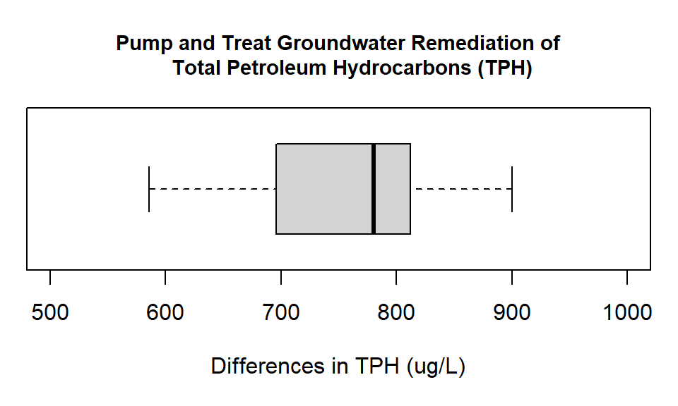
Figure 20.2: Box plot showing the differences in groundwater measurements of Total Petroleum Hydrocarbons (ug/L) at monitoring wells before and after pump and treat remediation.
From the horizontal boxplot it looks like our remediation was successful. All the differences are positive. Although, remember that for the test we do not use the actual data but the rank values.
Step 1: Set the Null and Alternate Hypotheses
Null hypothesis: There is no difference in the before and after measurements
Alternate hypothesis: There is a difference in the before and after measurementsStep 2: Implement the Wilcoxon test for paired data
Here we set the parameter:
paired=TRUEto indicate that we have a paired test, and we also set the parameterexact=FALSEto suppress the warnings. As always the alpha level is set at 0.05.with(TPH.remediation, wilcox.test(before, after, paired = TRUE, exact = FALSE)) #> #> Wilcoxon signed rank test with continuity correction #> #> data: before and after #> V = 45, p-value = 0.009 #> alternative hypothesis: true location shift is not equal to 0Step 3: Interpret the Results
From the output we see the \(\texttt{p-value = }\) 0.009152, which we would generally report as \(<0.001\), which is smaller than \(0.05\). So, we:
Reject the null hypothesis that the means are equal.In words: We have sufficient evidence to say the concentration of Total Petroleum Hydrocarbons is different after remediation. We know remediation had a positive effect by looking at the data values and the boxplot. That the remediation has had an impact is great news; but we still needs to be compare actual pollution levels to acceptable levels for the relevant land use, and understand things such as the cost effectiveness of the remediation. As always, the formal testing aspect is just a small part of the overall process.
20.3 Multiple Group: Kruskal-Wallis Test
The Kruskal-Wallis test is the non-parametric analogue of the familiar ANOVA for difference between means in multiple groups. The test examines the ranks of observations in the sample as a whole and measures how these ranks vary between groups in order to test whether or not all observations in the sample come from the same distribution.
For this example we will use the base R data set chickwts. The data set includes information on the weights of chickens fed six different types of feed, and the data is in long format. When data is in long format it means we have one continuous variable (weight) and one factor variable (feed) that has six levels. When working with multiple groups it is easiest to work with data in long format. What we are trying to do is help a farmer identify a feed which promotes the greatest weight gain in chickens.
Just as for the parametric approach, we start our investigation by looking at our data using the str() and summary() functions, and creating a boxplot. When the data are in long format if we want to get the quantile information that is plotted in the boxplot we use the tapply() function.
Note: This is the same data set used in the ANOVA R reference guide, so you can compare the different results.
# get summary & structure and create a boxplot of our differences
str(chickwts)
#> 'data.frame':    71 obs. of  2 variables:
#>  $ weight: num  179 160 136 227 217 168 108 124 143 140 ...
#>  $ feed  : Factor w/ 6 levels "casein","horsebean",..: 2 2 2 2 2 2 2 2 2 2 ...
summary(chickwts)
#>      weight           feed
#>  Min.   :108   casein   :12
#>  1st Qu.:204   horsebean:10
#>  Median :258   linseed  :12
#>  Mean   :261   meatmeal :11
#>  3rd Qu.:324   soybean  :14
#>  Max.   :423   sunflower:12
with(chickwts,tapply(weight,feed,quantile))
#> $casein
#>   0%  25%  50%  75% 100%
#>  216  277  342  371  404
#>
#> $horsebean
#>   0%  25%  50%  75% 100%
#>  108  137  152  176  227
#>
#> $linseed
#>   0%  25%  50%  75% 100%
#>  141  178  221  258  309
#>
#> $meatmeal
#>   0%  25%  50%  75% 100%
#>  153  250  263  320  380
#>
#> $soybean
#>   0%  25%  50%  75% 100%
#>  158  207  248  270  329
#>
#> $sunflower
#>   0%  25%  50%  75% 100%
#>  226  313  328  340  423
with(chickwts,boxplot(
  weight~feed,
  col= "lightgray",
  main= "",
  xlab= "Feed type",
  ylab= "Weight (g)",
  ylim= c(100,450),
  las= 1)
  )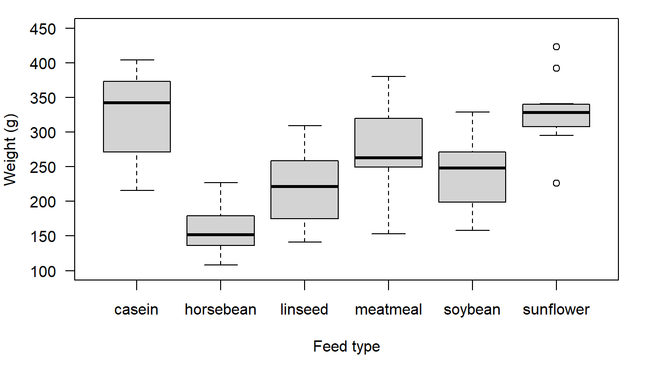
Figure 20.3: Chicken weight distributions for six different feed types.
Personally, I would be pretty comfortable with using an ANOVA test, but let’s say that because we only have between 10 and 14 observations per group we decide to use the non-parametric Kruskal-Wallis test rather than an ANOVA test.
There are no distributional assumptions with theKruskal-Wallis test, so we do not need the Bartlett test of constant group variance. Also, the test is not a test of differences in the group means, but rather is a test for some general kind of difference. The Null and Alternative hypothesis we use are therefore different to the Null and Alternative hypothesis used for the ANOVA test.
We use the function kruskal.test() to implement the Kruskal-Wallis test, and so for our formal test we have:
Step 1: Set the Null and Alternate Hypotheses
- Null hypothesis: The feeds all have the same effect on chicken weight gain
- Alternate hypothesis: The feeds do not all have the same effect on chicken weight gain
- Null hypothesis: The feeds all have the same effect on chicken weight gain
Step 2: Implement Kruskal-Wallis Test
When there is a tie in the rank values R will print a warning. This can be really annoying. The issue is trivial. In my experience the issue is at the 4th decimal place, and so I think it is to ignore these warnings. For reporting purposes we truncate our p-value reporting at p-value \(<0.001\), so there is never anything misleading in the way we report results. Unfortunately there is no easy way to turn off the warnings within the
kruskal.test()function, so for this test we just have to live with the warnings when they apply.with(chickwts, kruskal.test(weight ~ feed)) #> #> Kruskal-Wallis rank sum test #> #> data: weight by feed #> Kruskal-Wallis chi-squared = 37, df = 5, p-value = 5e-07Step 3: Interpret the Results
From the output we see the \(\texttt{p-value = }\) 5.113e-07; which we report as \(<0.001\). As the test p-value is smaller than \(0.05\) we:
Reject the null hypothesis that the feeds all have the same effect on chicken weight gain.
In our output we can also see that the \(\chi^2\)-statistic is 37.34. Technically, this is our test statistic and it is this value that our test p-value is based on. For decision making it is much easier to just focus on the p-value decision rule rather than working with test statistics, and that is what we do here.
Similar to the way we proceeded with the ANOVA example, given we reject the null, we now move on to try to identify the specific differences using pairwise comparisons.
20.3.1 Pairwise Comparisons
Recall the research question: which feed(s) should the farmer consider using if she wants heavier chickens. Here we will use the function pairwise.wilcox.test() to compare all feed types. Remember, for these pair-wise tests we are not looking for differences in the group means but just some general difference in the groups.
To implement the tests we use the pairwise.wilcox.test() function. The function works in a similar way to the the pairwise.t.test() function. Specifically, it calculates all the different possible combinations for us at once. This means we don’t need to type the wilcox.test() command 15 times (one for each pairwise combination). The pairwise.wilcox.test() also automatically adjusts the reported p-values to control the Type I error rate, which is important when conducting multiple comparisons.
The automatic adjustment to the p-values makes life easy for us as we can still apply our standard p-value decision rule to the results, where we know that the values have been adjusted to address the multiple comparison issue. This is something that only specialist software such as R is able to do, and it really saves a lot of time compared to the alternative of working through the adjustments manually. In all our testing we will rely on the default adjustment used by R, which is the holm adjustment.
Similar to when using the wilcox.test() function, when using the pairwise.wilcox.test() function it is possible to turn off the warnings by setting the parameter exact = FALSE. With pair-wise tests, it is possible to get a lot of warnings if you do not turn them off.
# Note i turn off the warnings using exact =FALSE
with(chickwts, pairwise.wilcox.test(weight, feed, exact = FALSE))
#>
#>  Pairwise comparisons using Wilcoxon rank sum test with continuity correction
#>
#> data:  weight and feed
#>
#>           casein horsebean linseed meatmeal soybean
#> horsebean 0.003  -         -       -        -
#> linseed   0.012  0.064     -       -        -
#> meatmeal  0.362  0.009     0.218   -        -
#> soybean   0.047  0.009     0.710   0.710    -
#> sunflower 1.000  0.002     0.003   0.347    0.014
#>
#> P value adjustment method: holm
As you probably suspected based on the boxplot, we have some significant differences between groups (e.g. horse bean and casein) and some non-significant differences (e.g meat meal and linseed). With reference to the boxplot, it can be seen that the two feeds that seem to have the highest distribution (i.e. they are the groups that feature at the top of the boxplot) are casein and sunflower. The test indicates no statistically significant difference for these groups. We also see meat meal, is also not significantly different from either casein or sunflower. So, it looks like the farmer has some options. She might now look to other factors such as cost or availability to decide what feed to provide her chickens. It is this final step that is important. The statistical test, whether it is a parametric test or a non-parametric test, is just one part of the process of working out what to do. You then typically need to look at other information – the boxplot and or the group means – to workout what you need to do.
20.3.2 Reporting Test Results
How you present numerical results in a table is just as important as how you present prepare figures. You must include information in a clear and concise way, without causing distraction with unnecessary information. Table 2 presents the results of our pair-wise comparisons, based on the non-parametric tests. For comparison purposes the results of the pair-wise t-tests are also shown in Table 3. Generally the p-values for the pair-wise t-tests (Table 20.2) are smaller.
| Casein | Horsebean | Linseed | Meatmeal | Soybean | |
|---|---|---|---|---|---|
| Horsebean | 0.003 | - | - | - | - |
| Linseed | 0.012 | 0.064 | - | - | - |
| Meatmeal | 0.362 | 0.009 | 0.218 | - | - |
| Soybean | 0.047 | 0.009 | 0.910 | 0.710 | - |
| Sunflower | 1.000 | 0.002 | 0.003 | 0.347 | 0.014 |
| Casein | Horsebean | Linseed | Meatmeal | Soybean | |
|---|---|---|---|---|---|
| Horsebean | \(<\) 0.001 | - | - | - | - |
| Linseed | \(<\) 0.001 | 0.094 | - | - | - |
| Meatmeal | 0.182 | \(<\) 0.001 | 0.094 | - | - |
| Soybean | 0.005 | 0.003 | 0.518 | 0.518 | - |
| Sunflower | 0.812 | \(<\) 0.001 | \(<\) 0.001 | 0.132 | 0.003 |
20.4 Bootstrapping as a modern solution
With modern computer power some people suggest non-parametric methods are no longer required. The ‘Bootstrap method’ is the alternative.
The idea with the Bootstrap is that we draw ‘samples’ from our initial sample, and then use these ‘samples’ to generate an implied distribution of sample mean.
You can download pre-baked code for R in the form of packages. The boot package will do some of the things the below code will do but not everything.
The below is an application of data science: combining computer code smartly to solve an applied statistics problem. Actually, the teaching team doesn’t have that much in computer science smarts, so I am pretty sure there are more efficient ways to code this. But it will work fast enough for any number crunching we will do.
First let’s create a dataframe to work with. Below we create both the full data set, and a test set.
# read in our data
tuna.data <- data.frame(
  Fish.cm = c(
193, 188, 185, 183, 180, 175, 170, 178, 173, 168, 165, 163),
Type = c("Males","Males", "Males","Males","Males","Males","Males",
          "Females","Females","Females","Females","Females")  )

# create some test data where I select just the Males
test.data <- with(tuna.data, Fish.cm[Type == "Males"])
test.data
#> [1] 193 188 185 183 180 175 170
The sample() function takes randomly selected values from the data set that you tell the function to sample from. If you set replace as true, each random draw is from the full data set. It we want to draw ten values we can do that as follows. The printed ten values have been randomly drawn from the underlying data set values.
sample(test.data, size =10, replace = TRUE )
#>  [1] 193 183 193 193 180 185 188 170 188 193
You can create blocks to hold numbers with the matrix() function. For example to create a block with four rows and seven columns that you can subsequently fill with numbers, you can use the code matrix( nrow = 4, ncol = 7, byrow = TRUE) to create the holding space.
You can then fill the matrix with values as follows, where in this example we fill the matrix (by row), with the values 1,…9 with something like: matrix(seq(1,9,1), nrow = 3, ncol = 3, byrow = TRUE).
Now let’s go back to our test.data. As we have seven observations in the test.data, we would fill a four by seven matrix with the same values in each row as follows.
test.samples.row <-
  matrix(test.data, nrow = 4, ncol = 7, byrow = TRUE)
test.samples.row
#>      [,1] [,2] [,3] [,4] [,5] [,6] [,7]
#> [1,]  193  188  185  183  180  175  170
#> [2,]  193  188  185  183  180  175  170
#> [3,]  193  188  185  183  180  175  170
#> [4,]  193  188  185  183  180  175  170
Now we can combine functions. The below code chunk says, draw 700 random values, from the test.data, and then fill up a matrix that is 100 rows long and 7 columns wide with the sample values, and save this object as m.test.samples. We can then look at some aspects of the object we have created.
Note that in addition to the mean and SD the values that represent the 95% of the distribution of means have also been calculated. In terms of testing, the 95% CI is important as we would not reject any values in the CI as plausible values for the null.
m.test.samples <- matrix(sample(test.data, size = 7*100, replace = TRUE),
                         nrow = 100, ncol = 7,  byrow = TRUE)

#  Next we create a series of the mean of each row.
test.sample.mean <- apply(m.test.samples, 1, mean)

mean(test.sample.mean) # mean
#> [1] 182
sd(test.sample.mean)  #sd
#> [1] 2.73
quantile(test.sample.mean, probs = c(0.025, 0.975)) #  95% confidence interval as:
#>  2.5% 97.5%
#>   176   187
It is also possible to plot the distribution of means. Both as a histogram, and as a density plot.
hist(test.sample.mean, main ="Bootstrap histogram")

plot(density(test.sample.mean), main = "Bootstap density curve ")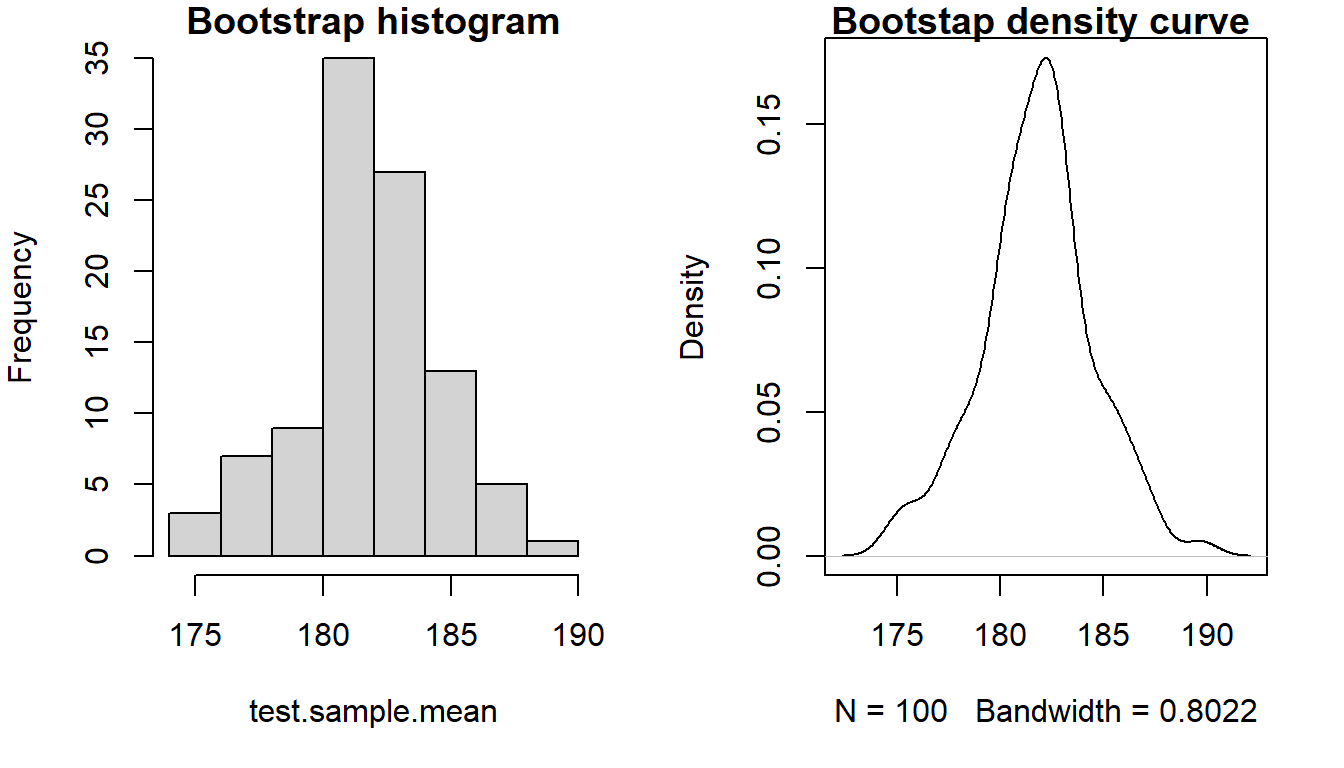
Figure 20.4: Distribution of bootstrap means.
Now to do the coding to work with some real data values. First, set the samples size you want, so you can change this easily later if needed, and then sample from our data set. Note that the length of the Male and Female sample is different.
no.samples=1000

f.samples <- with(tuna.data, matrix(sample(Fish.cm[Type == "Females"],
                 size = length(Fish.cm[Type == "Females"])*no.samples,
                 replace = TRUE),
                 nrow = no.samples,
                 ncol= length(Fish.cm[Type == "Females"]),
                 byrow=TRUE))

m.samples = with(tuna.data, matrix(sample(Fish.cm[Type == "Males"],
                size = length(Fish.cm[Type == "Males"])*no.samples,
                replace = TRUE),
                nrow = no.samples,
                ncol= length(Fish.cm[Type == "Males"]),
                byrow=TRUE))
Now I get the mean of each row all my samples. The code says read across each row of the data matrix and calculate the mean value, and save those value in an object called female.means and male.means. Next, for each sample I calculate the difference in the mean for each row and save those values in the object boot.stat. The final step is to derive the 95% Confidence Interval for my bootstrapped samples. This defines the do not reject zone. If zero is in this range I will not reject the null of no difference in the means of these sample.
female.means <- apply(f.samples, 1, mean)
male.means <- apply(m.samples, 1, mean)

boot.stat <- male.means - female.means

quantile(boot.stat, probs = c(0.025, 0.975))
#>  2.5% 97.5%
#>  5.43 19.91
Because zero is not in the 95% CI, I reject the null. Looking at the means, Male tuna are the larger fish
Now I create a plot to show my distribution, the 95% confidence interval, and the non-reject zone.
You really just want to run the code here as a block and look at the plot. This is starting to get advanced.
quant <- quantile(boot.stat, probs = c(0.025, 0.975))
boot.den <- density(boot.stat)
low.ci <- quant[1]
hi.ci<- quant[2]
x1b <- min(which(boot.den$x >= low.ci))
x2b <- max(which(boot.den$x <  hi.ci))
plot(density(boot.stat),
     main = "The bootstrap distribution",
     xlab = "Difference (Males - Females in cm")
with(boot.den, polygon(x=c(x[c(x1b,x1b:x2b,x2b)]),
                       y= c(0, y[x1b:x2b], 0),
                       border = "gray70",
                       col="gray70"))
legend("topleft", legend ="Do not reject zone", fill ="grey", bty ="n", border="grey", cex=0.8)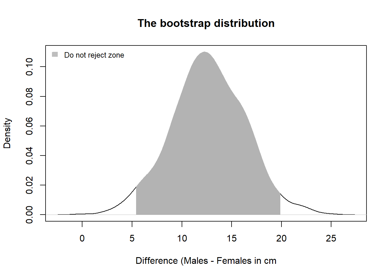
You can do the same thing for the medians. You just change the requested statistic.
female.meds = apply(f.samples, 1, median)
male.meds = apply(m.samples, 1, median)
boot.meds = female.meds - male.meds
quantile(boot.meds, probs = c(0.025, 0.975))
#>  2.5% 97.5%
#>   -23    -2
Given the above result it is possible to conclude from the 95% CI that we would reject the Null.
20.5 Non-parametric Regression
Non-parametric methods are also used in regression. So far we have seen regression models defined parametrically: for example a linear regression model is defined by the slope and the intercept parameters. Rather than assume a linear relationship, or a log-linear relationship, or any other parametric relationship between two variables, we can relax this assumption and have the form of the relationship be defined by the observed data. Such methods are robust to model mis-specification (e.g. assuming a linear relationship when in fact the relationship is of some other form). These methods are covered in more advanced courses.