Chapter 17 Analysis of Variance
The ANOVA (ANalysis Of VAriance) test is a classical statistical test associated with R. Fisher. The test is suited to situations where we have observations grouped by a categorical variable and we want to understand whether or not there are differences in the group means. The mathematical notation for ANOVA is horrible, but the intuition is relatively easy to understand.
The ANOVA test statistic follows the F-distribution, and large values are evidence against the null hypothesis that the group means are all the same. In practice we can think of the test as dividing the observed variation in the data into:
- The variation between the group means and the grand mean (the average across all the groups); and
- The variation within each group.
If the variation between the group means and the grand mean is high, and the variation within groups is small, this suggests there are true differences in the group means. On the other hand, if the variation between the group means and the grand mean is small, and the variation within groups is large, this suggests there are no real differences in the group means i.e. the variations we observe is just sampling variation.
For the ANOVA test, if we observe a p-value of less than 0.05 we say we have sufficient evidence to reject the null hypothesis that all the group means are the same. If we reject the null we then move on to pair-wise t-tests to try and determine which specific group means are different. For the pair-wise t-tests we use an adjustment method to control the Type I error rate. The need to adjust p-values to control the Type I error rate is one of the reasons we need specialist software.
If we observe a p-value that is greater than 0.05 we say we have insufficient evidence to reject the null hypothesis that all the group means are the same. If we do not reject the null hypothesis we do not proceed to pair-wise t-tests. We just stop our analysis at the ANOVA test. We have concluded that there are no significant differences so we stop.\
Similar to the case for the t-test, for the ANOVA test there are two possible formulas that we can use: one formula when the group variances are the same, and one formula for when the group variances are not the same. So, before we conduct an ANOVA test we have to conduct a pre-test to establish whether the group variances are the same or not. The test we use for this in the Bartlett test. If we reject the null for the ANOVA test we then go on to look for the specific differences between groups. This means that when we conduct an ANOVA test we usually have three tests to conduct:
- A Bartlett test to check whether the group variances are the same
- The actual ANOVA test (with either equal or unequal variance)
- Pair-wise t-tests, with an adjustment for multiple comparisons (if we reject the null for the ANOVA test).
We will work through these steps below. As with all previous statistical tests, we will set the alpha level at 0.05.
17.1 ANOVA - One Factor
For this example we will use the base R data set chickwts, which has the weights of chickens fed six different types of feed. The data is in long format. This means we have one continuous variable (weight) and one factor variable (feed) that has six levels. When working with multiple groups it is easiest to work with data in long format.
Let’s start by looking at our data and creating a box plot:
# get summary & structure and create a boxplot of our differences
str(chickwts)
#> 'data.frame':    71 obs. of  2 variables:
#>  $ weight: num  179 160 136 227 217 168 108 124 143 140 ...
#>  $ feed  : Factor w/ 6 levels "casein","horsebean",..: 2 2 2 2 2 2 2 2 2 2 ...
summary(chickwts)
#>      weight           feed
#>  Min.   :108   casein   :12
#>  1st Qu.:204   horsebean:10
#>  Median :258   linseed  :12
#>  Mean   :261   meatmeal :11
#>  3rd Qu.:324   soybean  :14
#>  Max.   :423   sunflower:12
with(chickwts,boxplot(weight~feed,
     col= "lightgray",
     main= "",
xlab= "Feed type", ylab= "Weight (g)", ylim= c(100,450), las= 1)) 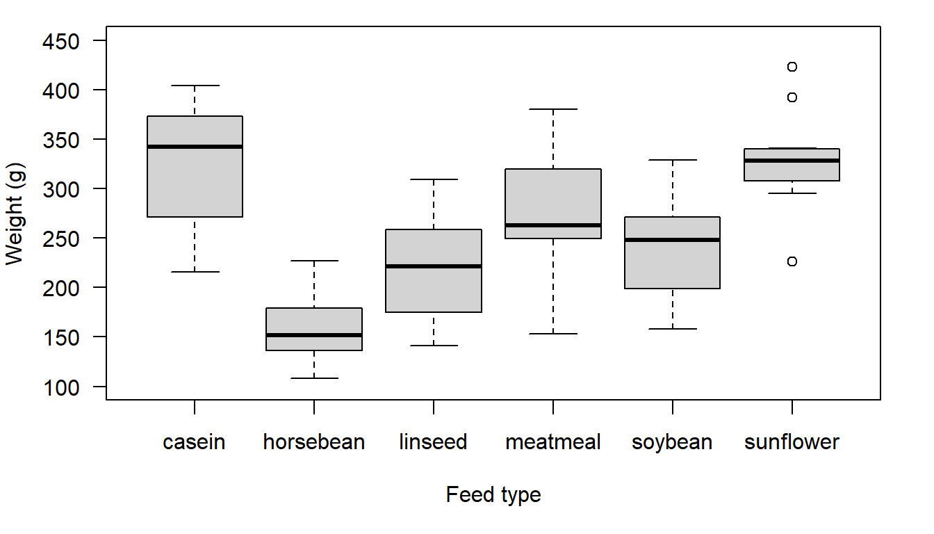
Figure 17.1: Chicken weight distributions for six different feed types
Based on the boxplot there look to be clear differences between at least some of the means, but it is not easy to see what the actual values are. Let’s use a new function, tapply(), to calculate the mean and standard deviation for each of our groups. Here you are applying the function mean() and sd() to the vector weight, grouped by feed. The tapply() function works when we have data in long format. The function generates results similar to the way results are generated using the pivot table function in MS Excel. Personally, I prefer to use MS Excel to work through data management issues, but you can do similar things with R.
with(chickwts, tapply(weight, feed, mean))
#>    casein horsebean   linseed  meatmeal   soybean sunflower
#>       324       160       219       277       246       329
with(chickwts, tapply(weight, feed, sd))
#>    casein horsebean   linseed  meatmeal   soybean sunflower
#>      64.4      38.6      52.2      64.9      54.1      48.8
As we saw in our boxplot, there is quite a difference between some of our group means, particularly horse bean on the lower end, and sunflower and casein on the higher end. What about our standard deviations? Remember, the standard deviation is the square root of the variance so the group standard deviations gives us an idea of whether the group variances are equal or not. The units of measurement for the standard deviation are just a bit easier to interpret than the units of measurement for the variance. Look carefully at the reported standard deviation values and also at the boxplot. Can you see the link between the visual display of the data and the group standard deviation values?
Now let’s formally test for equal variance across the groups. Because we have multiple groups the test we use is the Bartlett Test of Homogeneity of Variances. The Null hypothesis for the test is that the group variances are all equal; the Alternate hypothesis is that the group variances are not equal. The implementation of the test follows the standard format we use for most tests. First we use the with() function to direct R to the dataset we want to use. Next we use the bartlett.test() function to tell R what function to apply. Finally we specify the column names that contain the data we are working with. Although this explanation is quite brief, there is a separate reference guide on the Bartlett test that explains the steps in greater detail.
with(chickwts, bartlett.test(weight ~ feed))  # long data format, use ~ not ,
#>
#>  Bartlett test of homogeneity of variances
#>
#> data:  weight by feed
#> Bartlett's K-squared = 3, df = 5, p-value = 0.7
As the test p-value = 0.66, which is greater than 0.05, we do not reject the null hypothesis that the group variances are all equal: we have insufficient evidence to reject the null.
As such we set the parameter var.equal to TRUE in our ANOVA test of whether the groups means are the same.
Note: If we reject the null for the Bartlett test (i.e. we have a test p-value that is less than 0.05) when we conduct the ANOVA test we set the parameter var.equal to FALSE.
To implement the ANOVA test we use the function oneway.test(), and so for our formal test we have:
Step 1: Set the Null and Alternate Hypotheses
- Null hypothesis: The group means are all equal
- Alternate hypothesis: At least one group mean is different from the other groups
- Null hypothesis: The group means are all equal
Step 2: Implement Analysis of Variance Test
with(chickwts, oneway.test(weight ~ feed, var.equal = TRUE))
#>
#>    One-way analysis of means
#>
#> data:  weight and feed
#> F = 15, num df = 5, denom df = 65, p-value = 6e-10
Step 3: Interpret the Results
From the output we see the p-value = 5.936e-10; which we report as \(<\) 0.001. As the test p-value is smaller than 0.05 we:
Reject the null hypothesis that all the means are equal.
In our output we can also see the F-statistic (15.36). This is the statistic that our p-value is based on. For large numbers we reject the null.
So what now? If you were a farmer wanting to know which feed to give your chickens, which feed would you choose? You could decide from your boxplot, likely choosing casein or sunflower, but the figure doesn’t tell you if there is a feed which is statistically the highest, and the ANOVA test only tells you that the feeds are not ALL the same. This is where pair-wise comparisons can be helpful.
17.1.1 Pair-wise Comparisons
Let’s come back to our research question - which feed(s) should the farmer consider based on the weights of chickens eating that feed. Here we will use the function pairwise.t.test() to compare all our individual group means. With this function the parameter pool.sd is the equivalent of var.equal for the t.test(). We use the Bartlett test result to decide whether we set this parameter to TRUE or FALSE.
If we do not reject the null for the Bartlett test we set the parameter to TRUE. If we reject the null for the Bartlett test we set the parameter to FALSE. So, for this example we will set it to TRUE.
The pairwise.t.test() function does two things that make our life easy. First, it calculates all the different possible pair-wise combinations for us at once. Rather than having to type the t.test() command 15 times (one for each pair-wise combination) we just need to write one command. The second thing that the pairwise.t.test() command does for us is to automatically adjust the reported p-values to control the Type I error rate. The automatic adjustment makes life easy for us as we can still apply our standard p-value decision rule to the results, where we know that the values have been adjusted to address the multiple comparison issue. This is something that only specialist software such as R is able to do, and it really saves a lot of time compared to the alternative of working through the adjustments manually.
It is possible to use a variety of different adjustments for multiple comparisons. For example, by changing the parameter p.adjust.method and providing “none” for no adjustment (lower p-values), or “bon” for a more restrictive adjustment (higher p-values). The default adjustment used by R is the holm adjustment, and this is a good choice. As such we will not be changing this parameter value. So conducting all the required comparisons is quite easy.
with(chickwts, pairwise.t.test(weight, feed, pool.sd = TRUE))
#>
#>  Pairwise comparisons using t tests with pooled SD
#>
#> data:  weight and feed
#>
#>           casein horsebean linseed meatmeal soybean
#> horsebean 3e-08  -         -       -        -
#> linseed   2e-04  0.094     -       -        -
#> meatmeal  0.182  9e-05     0.094   -        -
#> soybean   0.005  0.003     0.518   0.518    -
#> sunflower 0.812  1e-08     8e-05   0.132    0.003
#>
#> P value adjustment method: holm
As you probably suspected based on the boxplot, we have some significant differences between groups (e.g. horsebean and casein) and some non-significant differences (e.g meat meal and linseed). The feeds with the two highest means, casein and sunflower, are not significantly different. We also see that the feed with the third highest mean, meat meal, is also not significantly different from either casein or sunflower. So, it looks like the farmer has some options in terms of the feed they select.
To make a final decision the farmer might now look to other factors such as cost or availability to decide what feed to provide her chickens. It is this final step that is important. The statistical test is just one part of the process of working out what to do. You then typically need to look at other information to workout what you actually need to do.
17.1.2 Reporting Test Results
How you present numerical results in a table is just as important as to how you present figures. You must include information in a clear and concise way, without causing distraction with unnecessary information. Table 17.1 presents the results of our pair-wise comparisons. This is a good format for you to follow.
| Casein | Horsebean | Linseed | Meatmeal | Soybean | ||
|---|---|---|---|---|---|---|
| Horsebean | <0.001 | - | - | - | - | |
| Linseed | <0.001 | 0.094 | - | - | - | |
| Meatmeal | 0.182 | <0.001 | 0.094 | - | - | |
| Soybean | 0.005 | 0.003 | 0.518 | 0.518 | - | |
| Sunflower | 0.812 | <0.001 | <0.001 | 0.132 | 0.003 |
17.2 The notation of the ANOVA model
The ANOVA test can be motivated by saying that when looking at grouped data the observed variation can be separated into two parts:
- The variation due to differences in the group means; and
- The variation of individual observations around each individual group mean.
The variation between group means is called the between group variation. The variation of individual observations around each individual group mean is called the within group variation.
The ANOVA test can be summarised with two propositions:
- If the variation due to differences in the group means is relatively
large, while the variation of observations around each group mean
is relatively small, it is likely there are true differences in the
group means. For this scenario the test will generate a small p-value.
- If the variation due to differences in the group means is relatively small, while the variation of observations around the group mean is relatively large, it is unlikely there are true differences in the group means. For this scenario the test will generate a relatively large p-value.
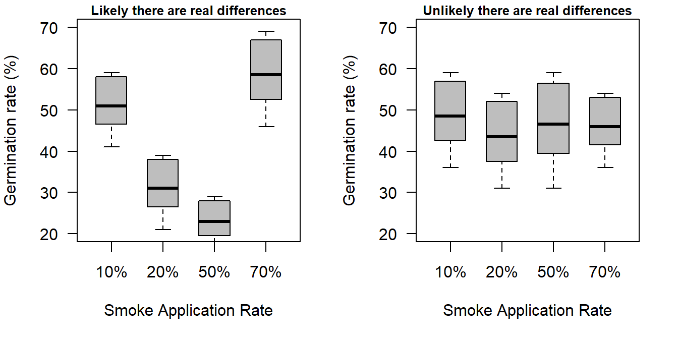
Figure 17.2: A comparison of where differences are likely and unlikely
If you understand the interpretation of the ANOVA test presented above you understand the fundamental element of ANOVA test. Unfortunately, the formal notation used to set out the ANOVA model is relatively intimidating. The complexity of the notation is one of the reasons a great many people refuse to come to terms with ANOVA. For the vast majority of people formal notation serves to obscure rather than highlight what is going on. The ANOVA model is especially bad in this respect. The type of notation used for ANOVA analysis will appear again and again throughout your studies. Because of this, a relatively formal introduction to ANOVA notation is presented below.
17.2.1 Introduction to notation
Consider the case where we have three groups. In group 1 we have 4 observations, in group 2 we have 5 observations, and in Group 3 we have 4 observations. That means we have something like the following:
For group 1 we have four observations: \(X_{1},X_{2}, X_{3},\text{ and }X_{4}\) which we summarise as \(X_{j}, j=1,\ldots,4\). For group 2 we have five observations: \(X_{1},X_{2},X_{3},X_{4},\text{ and } X_{5}\),which we summarise as \(X_{j}\), \(j=1,...,5\). For group 3 we have four observations: \(X_{1},X_{2},X_{3},\text{ and }X_{4}\) which we summarise as \(X_{j}\), \(j=1,...,4\). What you can see is that when we have groups of observations things get confusing if we use a single sub-script to index observations.
In the above expressions \(j\) was used to keep track of the number of observations in each group. To keep track of which group an individual observation belongs to we need to introduce a second subscript. This looks complex, but it we take things slowly it makes sense. When we have groups we use the notation \(X_{ij}\) to keep track of all the observations. The \(i\) tells us which group the observation belongs to and the \(j\) keeps track of the individual observations within each group.
So for the specific case we have:
- For group 1 we have: \(X_{11}\), \(X_{12}\), \(X_{13}\), and \(X_{14}\)
- For group 2 we have: \(X_{21}\), \(X_{22}\), \(X_{23}\), \(X_{24}\), and \(X_{25}\);
- For group 3 we have: \(X_{31}\), \(X_{32}\), \(X_{33}\), and \(X_{34}\).
The number of observations in each group can be different. In our example there are 4 observations in group 1 and group 3, but 5 observations in group 2. The indexation for j (the number of observations within each group) must reflect this, and so we write \(j=1,\ldots,n_{i}\). This says that the number of observations in group \(i\) runs from 1 through to the maximum number for group \(i\) , and so reflects the fact that the number of observations in each group can vary. In our example we have \(n_{1}=4\), \(n_{2}=5\), and \(n_{3}=4\).
We can denote the individual group means as \(\bar{X}_{1}\), \(\overline{X}_{2}\) , and \(\overline{X}_{3}\), and the average across all observations as \(\overline{X}_{G}\), which we call the grand mean. We know how to calculate these values. Formally, we write the group mean for group \(i\) as: \[\overline{X}_{i}=\frac{1}{n_{i}}\sum_{j}X_{ij}.\] This expression says, to find the mean for any given group, take all the observations for that group, add them up, and divide through by the total number of observations for that group. The expression \(\sum_{j}\) is read \(j\). So, if we take group 1 to illustrate we would have:
\[ \begin{aligned} \overline{X}_{1}&=\frac{1}{n_{1}}\sum_{j}X_{1j}\nonumber\\ &=\frac{1}{4}\left(X_{11}+X_{12}+X_{13}+X_{14}\right)\nonumber\\ &=\textrm{average for group 1.}\nonumber \end{aligned} \]
To find the overall grand mean for the data we know that we simply have to add up all the observations and divide through by the total number of observations. While in practice this is a simple operation in Excel or R, the formal notation is a little involved. First we have to implement a rule that will give us the total number of observations, which we will denote with \(N\) . The formal notation we use to denote the total number of observations is as follows:
\[ \begin{aligned} N&=\sum_{i}n_{i}\nonumber\\ &=n_{1}+n_{2}+n_{3}\nonumber\\ &=4+5+4\nonumber\\ &=13.\nonumber \end{aligned} \]
Now, we need a way to say add up in a sequence all the observations in group 1, group 2, and group 3. If we had a single group we could use the expression \(\sum_{j}X_{j}\) , which say add up all the observations indexed by \(j\). However, we need to say add up all the observations in group 1, group 2, and group 3. To see how this works let us start by writing out in full what we want to do. We want to write something that will say add up all 13 observations:
\(X_{11}+X_{12}+X_{13}+X_{14}+X_{21}+X_{22}+X_{23}+X_{24}+X_{25}+X_{31}+X_{32}+X_{33}+X_{44}\)
We know how to say add up all the values within a group. For group
1 we write this as \(\sum_{j}X_{1j}\), for group 2 we write \(\sum_{j}X_{2j}\),
and for group 3 we write \(\sum_{j}X_{3j}\). Now we want to add all
these values together so we have something that looks like:
\[\sum_{j}X_{1j} + \sum_{j}X_{2j} + \sum_{j}X_{3j}.\]
What we need is a second summation sign that says add up across the
groups. Formally we write \(\sum_{i}\sum_{j}X_{ij}\) if we want to
say add up all the observations from all groups. This expression says
add up all the observations in all groups; where the groups are indexed
by \(i\) and the individual observations within a group are indexed
by \(j\). For the three groups we have considered the term \(\sum_{i}\sum_{j}X_{ij}\)
translates as follows:
\[\sum_{i}\sum_{j}X_{ij}=X_{11}+X_{12}+X_{13}+X_{14}+X_{21}+X_{22}+X_{23}+X_{24}+X_{25}+X_{31}+X_{32}+X_{33}+X_{44}.\]
To find the average of the observations so we need to divide through by the total number of observation, which is \(N=\sum_{i}n_{i}\). So, formally we denote the grand mean as: \[ \begin{aligned} \overline{X}_{G}&=\frac{1}{N}\sum_{i}\sum_{j}X_{ij}\nonumber\\ &=\frac{1}{13}\left(X_{11}+X_{12}+X_{13}+X_{14}+X_{21}+X_{22}+X_{23}+X_{24}+X_{25}+X_{31}+X_{32}+X_{33}+X_{44}\right).\nonumber \end{aligned} \]
In terms of notation this is as complicated as things get, and we now have all the elements we need to consider a formal ANOVA model.
17.2.2 The ANOVA model
The proposition presented regarding the ANOVA test is that if the variation due to differences in the group means is relatively large, while the variation of observations around each group mean is relatively small it is likely there are true differences in the group means. The alternative contrasting scenario is one where the variation due to differences in the group means is relatively small, while the variation of observations around each group mean is relatively large it is unlikely there are true differences in the group means.\
The ANOVA test statistic is: \[\frac{\textrm{standardisied measure of between group variation}}{\textrm{standardisied measure of within group variation}}.\] This test statistic follows the \(F\)-distribution, and large values for \(F\) (p-value \(<\) 0.05) lead us to reject the null hypothesis of no differences between the groups. When adding up the differences between individual observations and the group mean, or differences between the group mean and the grand mean, positive and negative values will cancel out. To ensure that we have a positive value for the variation we therefore square each difference calculation.
17.2.3 Between group variation
We find the total between group variation for each group as the difference between the group mean and the grand mean multiplied by the number of observations in each group. This measure can be written as:
\(n_{1}\left(\overline{X}_{1}-\overline{X}_{G}\right)^{2}+n_{2}\left(\overline{X}_{2}-\overline{X}_{G}\right)^{2}+n_{3}\left(\overline{X}_{3}-\overline{X}_{G}\right)^{2}\).
In our example we have 4 observations in group 1, 5 observations in group 2, and 4 observations in group 3, so we have \(n_{1}=4\), \(n_{2}=5\), \(n_{3}=4\) or
\(4\times\left(\overline{X}_{1}-\overline{X}_{G}\right)^{2}+5\times\left(\overline{X}_{2}-\overline{X}_{G}\right)^{2}+4\times\left(\overline{X}_{3}-\overline{X}_{G}\right)^{2}\).
We can however also use the summation operator to write this in a formal way as: \(\sum_{i}n_{i}\left(\overline{X}_{i}-\overline{X}_{G}\right)^{2}\) = the total between group variation, and we call this measure the between group sum of squares. Note that the indexation subscript uses \(i\) as we are comparing group means to the grand mean. The standardisation we use is to divide through by the degrees of freedom. In a statistics context degrees of freedom works as follows. When we consider the sum of squares calculations there is a constraint that means if we have all but the last piece of information we are able to retrieve the final missing value. The final value is not free to take any value but rather is constrained to the value required by the formula we are using.
For our between group variation, if we know any \(k-1\) values we can retrieve the final value. The standardisation we use for the between group sum of squares is therefore \(k-1\). So, to summarise we have:\
\[\sum_{i}n_{i}\left(\overline{X}_{i}-\overline{X}_{G}\right)^{2} = \textrm{the between group sum of squares.}\]
We then have as our standardised measure of the between group variation: \[ \begin{aligned} \frac{\sum_{i}n_{i}\left(\overline{X}_{i}-\overline{X}_{G}\right)^{2}}{k-1} &=& \textrm{the standardised between group sum of squares}\nonumber\\ &=& \textrm{the between group mean squares.}\nonumber \end{aligned} \]
17.2.4 Within group variation
For the within group variation we have the same problem with positive and negative values that would cancel out, so again we square each deviation around the individual group means. The variation we want to add up is the variation of the individual observations around their respective group means. Specifically, the values that we want to add up are the following values:
\[ \begin{aligned} \textrm{Sum of squared deviations}&&\nonumber\\ \textrm{from group means}&=&\left(X_{11}-\overline{X}_{1}\right)^{2}+\cdots+\left(X_{14}-\overline{X}_{1}\right)^{2}+\nonumber\\ &&\left(X_{21}-\overline{X}_{2}\right)^{2}+\cdots+\left(X_{25}-\overline{X}_{2}\right)^{2}+\nonumber\\ &&\left(X_{31}-\overline{X}_{3}\right)^{2}+\cdots+\left(X_{34}-\overline{X}_{3}\right)^{2}\nonumber \end{aligned} \]
We know that we can write the sum of the squared deviations from the mean for the groups individually as:
- within group variation for Group 1 =\(\sum_{j}\left(X_{1j}-\overline{X}_{1}\right)^{2}\)
- within group variation for Group 2 =\(\sum_{j}\left(X_{2j}-\overline{X}_{2}\right)^{2}\)
- within group variation for Group 3 =\(\sum_{j}\left(X_{3j}-\overline{X}_{3}\right)^{2}\)
This means that we can, in the first instance pull together the information that describes the within group variation as: \[ \begin{aligned} \sum_{i}\sum_{j}\left(X_{ij}-\overline{X}_{i}\right)^{2}&=& \left(X_{11}-\overline{X}_{1}\right)^{2}+\cdots+\left(X_{14}-\overline{X}_{1}\right)^{2}+\nonumber\\ &&\left(X_{21}-\overline{X}_{2}\right)^{2}+\cdots+\left(X_{25}-\overline{X}_{2}\right)^{2}+\nonumber\\ &&\left(X_{31}-\overline{X}_{3}\right)^{2}+\cdots+\left(X_{34}-\overline{X}_{3}\right)^{2}\nonumber \end{aligned} \]
We call this the within group sum of squares. Within each group there
is one value that is not free to vary, and so the degrees of freedom
is equal to \(N-k\); the total number of observations minus the number
of groups. In the example we have been working with there are 19 observations
and 3 groups so we have 16 degrees of freedom. We then have as our
standardised measure of the within group variation:
\[
\begin{aligned}
\frac{\sum_{i}\sum_{j}\left(X_{ij}-\overline{X}_{i}\right)^{2}}{N-k}
&=& \textrm{the standardised within group sum of squares}\nonumber \\
&=& \textrm{within group mean squares.}\nonumber
\end{aligned}
\]
Again, technically this value is a variance estimate which follows
a chi-squared distribution.
The ANOVA test is then conducted as: \[F=\frac{\textrm{Between Group MS}}{\textrm{Within Group MS}},\] and we reject the null hypothesis of no significant difference in the group means if this value is large, where large is defined by the \(F\)-distribution (We use the fact that \(F\)-value, as the ratio of two chi-squared variables, follows the \(F\)-distribution).
In practice we need to know how to implement the test, and we can implement
the test in R using the oneway.test() function.